1.05 Counting the Uncountable: Sampling Biodiversity and Populations
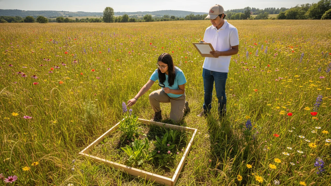
estimate population size by mark-recapture, calculate Simpson’s diversity index from quadrat samples, and use a computer model to explain how predator and prey populations affect each other.
- I can use mathematical representations, such as trends, averages, and graphs, to identify changes over time in the numbers and types of organisms in ecosystems of different scales.
- I can analyze mathematical representations to identify the most important factors that determine biodiversity and population numbers in an ecosystem.
- I can use evidence from mathematical representations to support explanations about how living and nonliving factors affect biodiversity and population size, and how ecosystems interact at different scales.
- I can describe, using models, how factors affecting ecosystems at one scale can cause observable changes in ecosystems at a different scale.
Phase 3: Make Sense
Warm-Up ~5 min
Do Now. The reserve board asks: “How many elk are there really, and are they changing the plants?” Nobody can count every animal in a mountain range or every plant in a meadow. Write one way you might estimate each.
Two meadows each have four plant species. Meadow A has 10 of each; Meadow B has 37 of one and 1 each of the others. Which is more diverse?
Instruction ~10 min
Why sample? Ecologists count a sample carefully and use mathematics to estimate the whole. HS-LS2-2 asks you to use these mathematical representations to explain what affects populations and biodiversity.
Mark-recapture. Capture a sample of animals, mark them harmlessly and release them. Later, capture a second sample and count how many are marked. If the marked animals have mixed evenly back into the population, the fraction marked in the second sample should equal the fraction of the whole population that is marked. The Lincoln-Petersen estimate is N ≈ MC/R, where M is the number marked in the first sample, C the size of the second sample and R the number of recaptures.
Worked example 1. Biologists mark 40 lizards; later they catch 50, of which 8 are marked. N ≈ 40 × 50 ÷ 8 = 250 lizards. The method assumes no births, deaths or migration between samples and that marks do not change an animal’s chance of being caught.
Measuring biodiversity. Biodiversity has two parts: richness (how many species) and evenness (how equally individuals are spread among them). Simpson’s diversity index combines both: D = 1 − Σn(n − 1) / [N(N − 1)], where n is the number of individuals of each species and N the total. D is the probability that two individuals picked at random belong to different species, from 0 (one species) toward 1 (very diverse).
Worked example 2. Quadrat A has four species with 10 plants each (N = 40). Σn(n − 1) = 4 × 90 = 360; N(N − 1) = 1,560; D = 1 − 360/1,560 ≈ 0.77. Quadrat B also has four species but 37, 1, 1 and 1 plants: Σ = 1,332; D = 1 − 1,332/1,560 ≈ 0.15. Same richness, very different diversity, because B is dominated by one species.
Lab procedure (schoolyard quadrats and bean mark-recapture), two periods.
- Choose two contrasting areas (for example a mowed lawn and an unmowed edge). Place a 1 m × 1 m quadrat at random in each area three times.
- In each quadrat, count the individuals of each plant type. Where you cannot name a plant, give it a code (species A, B, C) and photograph it.
- Calculate Simpson’s index for each area from the pooled counts.
- Mark-recapture model: take a scoop of beans from a bag, count them and replace them with the same number of colored beans (the “marked” animals). Shake the bag well.
- Take a second scoop, count the total and the colored beans, and calculate N = MC/R. Repeat three times and average.
- Count every bean in the bag and compare the true size with your estimates.
| Area | Species (codes) | Counts per species | Total N | Simpson’s D |
|---|---|---|---|---|
| Area 1 | ||||
| Area 2 |
| Trial | Marked (M) | Second sample (C) | Recaptured (R) | Estimate N = MC/R |
|---|---|---|---|---|
| 1 | ||||
| 2 | ||||
| 3 |
Illustrative field data (if you cannot sample). Three quadrats pooled in each of two areas of one school site. These are constructed teaching data, not a real survey. Area 1, mowed lawn (N = 200): perennial ryegrass 142, white clover 31, annual bluegrass 18, dandelion 9. Area 2, unmowed fence line (N = 135): wild oat 34, field poppy 21, filaree 19, bur clover 17, yarrow 12, black mustard 11, broadleaf plantain 9, red fescue 8, wild onion 4. Bean model, true population 250: M = 40; second scoops of 50 with 8 colored, 60 with 11 colored, and 45 with 6 colored. As a check, Area 1 comes out near 0.46 and Area 2 near 0.86, and the mean of the three estimates lands close to, but not exactly on, 250.
Why diversity matters. A diverse ecosystem usually has more pathways for energy and matter, so the loss of one species is less likely to cause a collapse. Unit 2 tests that idea on kelp forests.
Predators and prey in a model. Populations are linked. More prey means more food for predators, so predators increase; more predators eat more prey, so prey decrease; then predators starve and decrease, and prey recover. The Wolf Sheep Predation model in NetLogo Web runs this with simple rules for each animal, and with grass turned on it adds a resource that limits the sheep. By changing one parameter at a time, you can test what makes the system stable and what makes it collapse.
Reading: OpenStax Biology 2e, Chapter 45 (Population and Community Ecology) and Chapter 46 (Ecosystems), CC BY 4.0.
Guided Exercises ~15 min
Calculate, then test the model.
Independent Practice ~10 min
Analysis questions.
Which area is more diverse? Is the difference due to richness, evenness or both? Cite your indexes and counts, and propose one human action that would change Area 1's diversity, predicting the effect on Simpson's index.
How close was your mark-recapture mean to the true count? Explain why the average of three trials is more reliable than one, and how the board could use the quadrat method to check whether elk grazing is changing plant diversity.
Closure ~5 min
We can now count, measure diversity and model linked populations. Next: we pull the unit’s science into one revised model of the herd.
Exit ticket: a reserve's grazed plot has D = 0.40 and an ungrazed plot D = 0.80. Write one claim the data support and one question they raise.
How confident are you that you can estimate a population by mark-recapture and calculate a diversity index from sample data?
Teacher notes
Timing: two 50-minute periods: day one for fieldwork and the bean model, day two for calculations and the NetLogo model.
Materials: quadrat frames (meter sticks or string and pegs), clipboards, tally sheets, a paper bag with a known number of white beans, colored beans for marking, devices for NetLogo Web.
Options: students who cannot do fieldwork use the illustrative field data; any two contrasting patches of a park, yard or sidewalk strip work.
Listen for: “more species always means higher D”; forgetting the −1 terms; assuming mark-recapture is exact.
Support / stretch: give a spreadsheet with n(n − 1) columns. Stretch: calculate the Shannon index for the same data and compare the ranking.