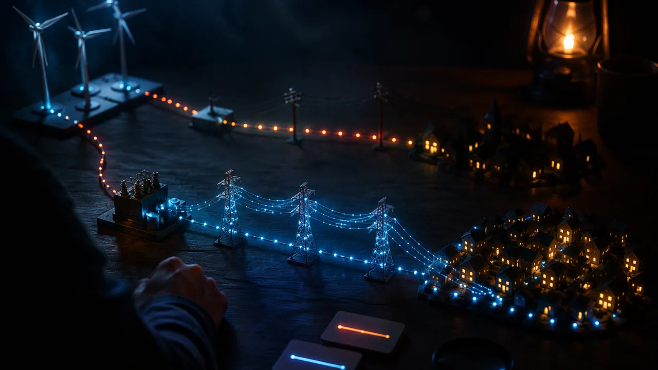
use a circuit simulation to model the impact of proposed transmission designs on the energy delivered from a wind farm, evaluate them against weighted criteria and trade-offs, and explain the physics of generation, transformation and loss.
Instruction
The engineering problem. Missouri’s largest wind farms stand in Atchison County, in the state’s northwest corner, where the U.S. Geological Survey counts 342 turbines with 800 MW of capacity, far from St. Louis and Kansas City. Wind power also crosses the state: in 2023 the Missouri Public Service Commission approved an amended certificate for the Grain Belt Express, an approximately 800-mile, ±600 kV direct-current line to carry Kansas wind power east, with a converter station in Monroe County delivering 2,500 MW into Missouri. You will model a transmission link from a wind farm to a town, test proposed solutions in a circuit simulator (9-12.ETS1.B.2), and recommend a design that balances energy losses against cost and other criteria (9-12.ETS1.B.1).
A tabletop-scale model in Falstad. The Falstad circuit simulator (a free web app) lets you build AC circuits with transformers and read currents, voltages and power. Scale model (illustrative): a 12 V AC source is the wind farm, a 10 Ω resistor is the long line, and a 10 Ω resistor is the town.
- Direct connection: I = 12/(10 + 10) = 0.60 A. The town gets I2R = 3.60 W and the line wastes 3.60 W: 50% delivered.
- With a 1:10 step-up and a 10:1 step-down transformer (ideal): the line runs at 120 V. Seen from the line, the town’s 10 Ω looks like 10 × 102 = 1,000 Ω, so the line current is 120/(10 + 1,000) = 0.1188 A. The line wastes 0.141 W and the town gets 14.12 W: 99.0% delivered.
Same line, same town, but raising the transmission voltage by 10 cut the line current by about 5 and the fraction lost from 50% to 1.0%. In the full-scale version from Lesson 3.4, 500 kV instead of 115 kV cut losses from 7.6% to 0.4% of 100 MW.
Proposed solutions to test. Each changes one thing: (1) a higher transmission voltage; (2) a thicker conductor (lower R, but heavier and costlier towers); (3) a shorter route (lower R, but crossing more sensitive land); (4) local battery storage at the town that smooths demand, lowering the peak current. Model each by changing the matching element in the simulator and record the delivered fraction.
Criteria and constraints. Criteria: fraction of energy delivered, reliability, cost, land and wildlife impact, and severe-weather risk (ice storms and high winds that bring lines down). Constraints: budget, available right-of-way, and safety clearances that grow with voltage. Higher voltage cuts losses but needs taller towers, bigger insulators and wider clearances. A weighted decision matrix makes those trade-offs explicit. Be honest about what the model leaves out: real lines also have reactance, transformers are not ideal, and the numbers here are illustrative.
What the physics must show. Your report explains, with fields, how the turbine’s generator converts kinetic energy to electrical energy (Faraday’s law), how transformers change voltage, and why I2R makes high voltage efficient.
📖 Read for this lesson
The reading opens over the lesson; close it to come back to exactly where you were. The checks below draw on it.
Formative check
Work through these before moving on. They are not graded — they tell you whether the standard below has landed yet.
Simulation & tools
Transmission with and without transformers
Open the Falstad simulator (Circuits menu → blank circuit). Build (a) a 12 V AC source in series with a 10 Ω line resistor and a 10 Ω load. Hover over each resistor to read its power. Then build (b) the source feeding a 1:10 transformer, the 10 Ω line, a 10:1 transformer and the 10 Ω load. Record the line current, line power and load power in both. Compare with the lesson’s predictions (3.60 W and 0.141 W lost). Then test one proposed solution of your own. No device: compute both cases by hand as the lesson does and add a third case with a 1:20 ratio.
Open Falstad Circuit Simulator (Paul Falstad) ↗ · Falstad Circuit Simulator (Paul Falstad) · GPL open source
Raising the transmission voltage by a factor of 10 (for the same delivered power) changes the line’s I2R loss by what factor?
If the simulation shows 99% delivery with transformers, the real line will also deliver 99%.
How confident are you that you can use a simulation to test transmission designs and defend a recommendation with physics and trade-offs?
Unit 3 checkpoint
Do this before you start the task. It covers the whole unit and tells you what to review first.
Two +2.0 μC charges 0.30 m apart repel with N.
If the distance between two charges is halved, the force
A 1 V potential difference gives each coulomb 1 J of energy.
A 470 Ω resistor across 9.4 V carries mA.
In a series circuit, which quantity is the same for every resistor?
200 Ω and 300 Ω in parallel have an equivalent resistance of Ω.
Which observation is the strongest evidence that a current produces a magnetic field?
A wire carrying 3.0 A makes a field of μT at 1.0 cm.
A strong magnet held still inside a coil keeps inducing a current.
Why does the grid transmit power at high voltage?
A transformer with 100 primary and 2,000 secondary turns on 12 V AC gives V.
Testing four transmission designs in a circuit simulator before choosing one is an example of using a computer simulation to model the impact of proposed solutions.
Design Report: Wind to Wire
Task: Recommend a transmission design to carry energy from a Missouri wind farm, such as those in Atchison County, to a town. In the Falstad simulator (or by hand calculation, an equal-credit route), model a baseline link and at least three proposed solutions (for example a higher transmission voltage, a thicker conductor, a shorter route or local storage), recording the delivered fraction for each. Scale your best result up with I = P/V and I2R for a 100 MW link, labeling every input as sourced or illustrative. Build a weighted decision matrix with at least four criteria (energy delivered, cost, land and wildlife impact, severe-weather risk, reliability) and the constraints you must respect. Explain the physics from wind to outlet: Faraday’s law in the generator, the transformer turns ratio, and why the loss depends on the square of the current. State the limits of your model.
Submission workflow
- Stage 1 — Plan. The problem, criteria and constraints with weights, the baseline model and the solutions you will test.
- Stage 2 — Reviewed draft. After a day’s break, rebuild one of your circuits from scratch (or recompute it by hand), recheck your scale-up calculation, and argue against one of your own weights; if a parent, guardian or other adult reader is willing, have them check the calculation with you. Submit the review notes and your revision plan.
- Stage 3 — Revised final. 1,000-1,400 words with simulation screenshots or hand calculations, a results table, the decision matrix, the physics explanation and the model’s limits.
- Stage 4 — Presentation or defense. Five minutes, recorded on video or audio (a written defense earns equal credit): your recommendation, the evidence, one trade-off, and your answers to two questions about your model, such as “What does your model leave out?” and “Would your recommendation change if cost mattered most?”
How it is scored
| Criterion | What proficient looks like |
|---|---|
| Simulation of solutions (9-12.ETS1.B.2) | Builds a working baseline model and tests at least three solutions, recording comparable results. |
| Trade-off evaluation (9-12.ETS1.B.1) | Weighted criteria and constraints, correct arithmetic, and a recommendation that follows from them. |
| Induction and fields (9-12.PS2.B.2, 9-12.PS3.C.1) | Explains generation and transformers with Faraday’s law and field ideas. |
| Energy accounting (CCC.5, MP.4) | Correct I = P/V and I2R calculations with units, scaled from model to grid. |
| Sources and limits (RST.11-12.7) | Inputs sourced or labeled illustrative; model limits stated. |
| Defense (SEP.6) | Clear recommendation and reasoned answers to questions. |
Wind to Wire, Worked by Hand: Every Proposed Solution, the Scale-Up and a Filled Decision Matrix
SLS worked model of the Lesson 3.5 transmission link (illustrative resistances and scores), with line voltages, route lengths and converter capacity from the Missouri Public Service Commission’s Report and Order in File No. EA-2023-0017 (Grain Belt Express LLC, issued Oct. 12, 2023, effective Nov. 11, 2023), as posted by the U.S. Department of Energy; retrieved Nov. 5, 2026 · SLS original, with Missouri Public Service Commission figures (public record)
Why this reading. The task says the hand-calculation route earns equal credit with the simulator, but the lesson works only two cases. Here are all the cases the task names, worked by hand in one table, so that the results table, the scale-up and the decision matrix can be built without any software, and so that a simulator run can be checked line by line. The transmission figures used for scale-up are sourced; everything marked illustrative is a teaching number.
1. The model and how each case is computed
Source 12 V AC (the wind farm), a line resistance Rline, a town resistance Rtown. With ideal transformers of turns ratio r (step up by r at the farm, down by r at the town), the line runs at 12r volts and the town looks, from the line, like r2Rtown. Line current I = 12r/(Rline + r2Rtown); line loss I2Rline; power to the town I2r2Rtown; delivered fraction = town ÷ (town + line).
Table 1. Baseline and six proposed solutions (illustrative model)
| Case | Line current (A) | Line loss (W) | Town power (W) | Delivered |
|---|---|---|---|---|
| Baseline: direct, 12 V, 10 Ω line, 10 Ω town | 0.6000 | 3.600 | 3.60 | 50.0% |
| 1:10 step-up and 10:1 step-down | 0.1188 | 0.141 | 14.12 | 99.0% |
| 1:20 step-up and 20:1 step-down | 0.0599 | 0.036 | 14.33 | 99.8% |
| Thicker conductor: line 5 Ω, no transformers | 0.8000 | 3.200 | 6.40 | 66.7% |
| Shorter route: line 7 Ω, no transformers | 0.7059 | 3.488 | 4.98 | 58.8% |
| Thicker conductor with 1:10 transformers | 0.1194 | 0.071 | 14.26 | 99.5% |
| Local storage: peak town load halved (20 Ω), no transformers | 0.4000 | 1.600 | 3.20 | 66.7% |
The baseline reproduces the lesson: 0.60 A, 3.60 W lost, 3.60 W delivered, 50%. The 1:10 case reproduces it too: 120 V on the line, 0.1188 A, 0.141 W lost, 14.12 W delivered, 99.0%. Note what each solution does to the amount delivered as well as the fraction: the transformer cases deliver four times the baseline power to the same town because the line no longer throttles the current; the thicker and shorter lines raise both the fraction and the amount; local storage (a town that draws half the peak current because a battery supplies the rest) raises the fraction to 67% but the town takes less from the line. Halving Rline at 1:10 changes the delivered fraction from 99.0% to 99.5%, a small gain on top of a large one; the voltage did most of the work.
2. Scaling up: a 100 MW link
Sourced inputs. Missouri’s own long-distance wind line is described in the Missouri Public Service Commission’s Report and Order of October 12, 2023 (File No. EA-2023-0017, effective November 11, 2023), which amended the certificate of the Grain Belt Express: “an approximately 800-mile, overhead, multi-terminal ±600 kilovolt (kV) high-voltage, direct current (HVDC) transmission line.” Per the order, the line runs about 370 miles from a converter station near Dodge City, Kansas, to the Missouri border and about 156 miles across Missouri to a converter station in Monroe County, which was enlarged “from 500 MW to 2500 MW”; a roughly 40-mile AC line, the “Tiger Connector,” links it to Ameren Missouri’s 345 kV system. The Commission found that HVDC “can transfer significantly more power with lower line losses over longer distances than comparable AC lines.” Illustrative input: a line resistance of 10 Ω (the lesson’s figure; real resistance depends on conductor size, length and temperature, and is not sourced here).
| Transmission voltage | Current for 100 MW, I = P/V | Loss in 10 Ω, I2R | Loss as a share of 100 MW |
|---|---|---|---|
| 115 kV | 870 A | 7.56 MW | 7.6% |
| 345 kV (Ameren Missouri’s AC line that the Grain Belt converter feeds) | 290 A | 0.84 MW | 0.8% |
| 500 kV | 200 A | 0.40 MW | 0.4% |
Raising the voltage by 10 for the same delivered power cuts the current by 10 and the loss by 100: the quiz’s factor of 1/100. Grain Belt’s full 2,500 MW at 345 kV would need 2,500,000,000 ÷ 345,000 = 7,246 A. Treated simply as a 600 kV line it needs 4,167 A; a ±600 kV line actually has two conductors (poles) at +600 kV and −600 kV, 1,200 kV apart, so the current is 2,500,000,000 ÷ 1,200,000 = 2,083 A, and for the same conductor the I2R loss is (7,246/2,083)2 = 12.1 times smaller than at 345 kV.
Why the model has transformers but Grain Belt has converters. A transformer works only with a changing current (Faraday’s law needs a changing flux), so the grid is AC. A DC line cannot use transformers; instead, converter stations at each end turn AC into DC and back with power electronics. The PSC order notes that the project will use voltage-sourced converter technology. Your Falstad model uses AC and transformers, which is right for an AC link from a wind farm to a town; say so in your report if you mention Grain Belt.
3. A decision matrix with the numbers filled in (illustrative weights and scores)
Scores 1 (worst) to 5 (best), multiplied by the weight. Cost, land and severe-weather scores are judgments explained in the basis column, not measurements; your report may weight them differently and must say why.
| Criterion (weight) | Baseline | Higher voltage | Thicker conductor | Shorter route | Local storage | Basis |
|---|---|---|---|---|---|---|
| Energy delivered (4) | 1 | 5 | 3 | 2 | 3 | delivered fraction and amount, Table 1 |
| Cost (3) | 5 | 2 | 3 | 3 | 2 | taller towers and bigger insulators; heavier conductor; land purchase; batteries |
| Land and wildlife impact (2) | 4 | 3 | 4 | 1 | 4 | wider clearances at high voltage; a shorter route crosses the sensitive land the long one avoided |
| Severe-weather risk: ice storms and high winds (3) | 3 | 3 | 4 | 3 | 4 | taller high-voltage towers catch more wind and ice load; a heavier conductor on stronger towers rides out ice loads better; storage keeps the town supplied when a line comes down |
| Reliability (2) | 2 | 4 | 3 | 3 | 5 | a stored reserve rides through outages |
| Weighted total | 40 | 49 | 47 | 34 | 48 |
Higher voltage leads local storage by a single point on these weights, with the thicker conductor one point further back: three solutions within two points of each other. That is not a failure of the matrix; it is the finding. The recommendation then turns on the constraint you cannot score: whether the right-of-way and the budget allow 500 kV towers. State which constraint decided it.
4. What the model leaves out
Real lines have reactance as well as resistance, so current and voltage are not in step and some of the current does no useful work; real transformers lose 1–2% each as heat; conductor resistance rises with temperature, so a line carries less on a hot Missouri summer afternoon; and the wind farm’s output is not a steady 12 V. None of that changes the direction of the results in Table 1, and all of it changes the exact numbers. A report that scales 99.0% to a real line without saying so has claimed more than the model can support.
Your turn
- Recompute rows 1, 2 and 3 of Table 1 by hand, showing the reflected town resistance r2Rtown in each.
- Add a case of your own (for example 1:10 transformers with a 20 Ω storage-assisted town) and place it in the table.
- Compute the current and the 10 Ω loss for Grain Belt’s 2,500 MW at 345 kV, and explain why a real line of that capacity uses several conductors per phase (or several lines).
- Re-weight the matrix with severe-weather risk at 5 and cost at 1, and report whether the recommendation changes.
Sources: Missouri Public Service Commission, Report and Order, File No. EA-2023-0017 (Grain Belt Express amended CCN), Oct. 12, 2023 (energy.gov)