measure brine shrimp hatching success across a range of salinities, identify the range of tolerance, and use the results to explain how changing salinity, such as road salt washing into a Missouri creek, affects populations and ecosystems.
Instruction
Every organism has a range of tolerance. For any environmental factor, such as temperature, salinity or pH, a species survives and reproduces well within an optimal range, poorly in the zones of stress on either side, and not at all beyond its limits. When conditions shift, the populations of some species grow, others shrink, and the ecosystem can change. This lab lets you measure a tolerance curve directly.
Missouri’s changing salinity. Salinity is measured in parts per thousand (ppt), grams of salt per liter of water. Seawater is about 35 ppt; Missouri’s rivers and creeks are fresh water, close to 0 ppt. But every winter, crews spread deicing salt, mostly sodium chloride, on roads, and meltwater carries it into storm drains and creeks. Scientists at the U.S. Geological Survey’s research center in Columbia sampled Hinkson Creek during snowmelt, when the creek was low. At one site the water held 1,252 milligrams of chloride per liter, more than five times the 230 mg/L the U.S. Environmental Protection Agency recommends as a long-term limit for aquatic life. A tiny freshwater crustacean, the water flea, survived 30 percent of the time in that water, compared with 100 percent in clean creek water, and produced far fewer young. That much chloride is only about 2 ppt of salt. Freshwater animals have tolerance curves that sit far below the brine shrimp’s.
The organism. Brine shrimp (Artemia) are tiny crustaceans whose eggs, called cysts, can survive drying for years and hatch within a day or two in salt water. They are sold as fish food and are safe and inexpensive. Hatching success, the percentage of cysts that hatch, is a simple, countable measure of how well a salinity suits the species.
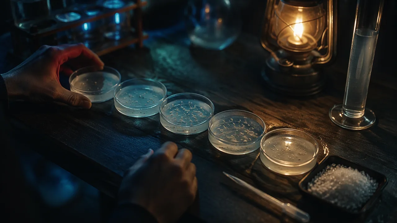
Designing a fair test. Make solutions from non-iodized salt: 10 g of salt in 1 L of water is 10 ppt. The independent variable is salinity; the dependent variable is the percentage hatched. Control temperature, light, water volume and the number of cysts per container. Counting all the cysts is slow, so count a sample: place a measured drop on a slide or dish, count hatched nauplii (larvae) and unhatched cysts, and calculate the percentage.
Reading an illustrative result. In an illustrative data set, 50 cysts per salinity were counted after 48 hours: 2 hatched in 0 ppt (4%), 21 in 10 ppt (42%), 34 in 20 ppt (68%), 41 in 35 ppt (82%), 30 in 50 ppt (60%) and 9 in 80 ppt (18%). The curve rises, peaks near seawater salinity, and falls on both sides. A salt lake moving from 35 ppt toward 80 ppt would still support some brine shrimp, but far fewer, with effects on every bird that feeds on them. A creek’s animals face the same shape of curve at much lower salinities. That is the kind of evidence 9-12.LS2.C.1 asks you to evaluate.
📖 Read for this lesson
The reading opens over the lesson; close it to come back to exactly where you were. The checks below draw on it.
Lab: Brine shrimp hatching across salinities
Question. How does salinity affect the hatching success of brine shrimp, and what range of salinity do they tolerate?
Materials
- Brine shrimp cysts (aquarium or pet store, or online), about 1/4 teaspoon in all
- Non-iodized salt, a kitchen scale or measuring spoons, and dechlorinated water (tap water left out overnight, or bottled spring water)
- Six clear cups or jars labeled 0, 10, 20, 35, 50 and 80 ppt, a desk lamp and a thermometer
- Droppers or drinking straws, a magnifying glass or a phone camera zoomed in, and a white saucer or lid as a counting surface
- Tell a parent or guardian before you start; wear safety glasses or goggles when mixing and pouring salt solutions, and rinse eyes with water if splashed. Never taste a solution.
- Wipe spills immediately to prevent slips, and keep water away from the lamp and its cord.
- Treat the brine shrimp humanely; at the end, feed them to a home aquarium fish or pour them onto garden soil. Never release them into a creek, pond or storm drain.
Procedure
- Make 200 mL of each salt solution (for example, 7 g of salt in 200 mL of water is 35 ppt). Label each cup and record its temperature.
- Add a small, equal pinch of cysts to each cup (about 50 to 100 cysts). Place all cups under the same lamp at the same distance.
- After 24 hours, gently swirl each cup and look for swimming nauplii. Record observations.
- After 48 hours, take three drops from each cup onto the white saucer, count hatched nauplii and unhatched cysts with the magnifying glass or a zoomed phone photo, and calculate the percentage hatched.
- Average your three counts for each salinity and record the means in your data table.
- Graph percentage hatched against salinity and mark the optimal range and the zones of stress.
Data
| Salinity (ppt) | Hatched | Unhatched | % hatched (mean of 3 drops) | Observations |
|---|---|---|---|---|
| 0 | ||||
| 10 | ||||
| 20 | ||||
| 35 | ||||
| 50 | ||||
| 80 |
Analysis
- Describe the shape of your tolerance curve and identify the optimal range. Cite at least three data points.
- Use the Hinkson Creek water flea results in this lesson and its reading. Compare the water flea’s response to salt with your brine shrimp curve, then predict how a winter of heavy road salting would affect a creek population with a similar tolerance curve, and what other organisms in that food web would feel the effect.
- Identify the controlled variables and one variable you could not fully control. How might it have affected your results?
- Why is hatching success only one part of a species’ response to salinity? Suggest a second measurement.
If you cannot do this lab in person: Use the illustrative data set in the lesson (hatching percentages at six salinities) and the drop-by-drop counts in this lesson’s reading to build the curve and complete the analysis.
Formative check
Work through these before moving on. They are not graded — they tell you whether the standard below has landed yet.
At 50 ppt, 30 of 50 cysts hatched, a hatching success of %.
How many grams of salt make 500 mL of a 35 ppt solution?
If a lake’s salinity rises beyond a species’ optimal range, the species may persist but with lower reproduction, which can reduce food for its predators.
Chloride in Hinkson Creek peaked during winter snowmelt, when the creek was low. Which is the best explanation?
How confident are you that you can measure a tolerance curve and use it to explain how changing conditions affect populations?
Practice
Work these on paper or in your notebook, then open Check your answer. Aim for all of Fluency and Application; try at least one Challenge.
Printable version: this unit’s practice workbook (PDF)
Fluency
Build speed and accuracy with the core skill.
- How many grams of salt make 200 mL of a 35 ppt solution?
Check your answer
Answer: 7 g35 g per liter × 0.2 L = 7 g. - How many grams of salt make 500 mL of a 10 ppt solution?
Check your answer
Answer: 5 g10 × 0.5 = 5 g. - How many grams of salt make 250 mL of an 80 ppt solution?
Check your answer
Answer: 20 g80 × 0.25 = 20 g. - 41 of 50 cysts hatched at 35 ppt. What is the hatching success?
Check your answer
Answer: 82%41 ÷ 50 = 0.82.
Application
Use the skill in context. Show your reasoning.
- 1 L of 35 ppt seawater is mixed with 1 L of fresh water. What is the salinity of the mixture? What if 3 L of seawater is mixed with 1 L of fresh water?
Check your answer
Answer: 17.5 ppt; about 26.3 ppt35 g in 2 L = 17.5 g/L; 105 g in 4 L = 26.25 g/L. - Snowmelt water at one Hinkson Creek site in Columbia held 1,252 mg/L of chloride. (a) How many times the EPA chronic criterion of 230 mg/L is that? (b) Chloride is about 60.7% of the mass of sodium chloride. If all of it came from road salt, about how many ppt of salt is that?
Check your answer
Answer: (a) About 5.4 times; (b) about 2.1 ppt(a) 1,252 ÷ 230 = 5.44. (b) 1,252 ÷ 0.607 = 2,063 mg/L ≈ 2.06 g/L ≈ 2.1 ppt. - Using the illustrative hatching curve (82% at 35 ppt, 60% at 50 ppt, 18% at 80 ppt), predict the effect on birds that feed on brine shrimp if a lake’s salinity rises from about 50 to about 80 ppt.
Check your answer
Answer: Hatching success falls from about 60% to about 18%, a drop of about 70% in new shrimp, so birds would find much less food and the lake could support fewer of them.(60 − 18) ÷ 60 = 0.70; the effect passes up the food web.
Challenge
Stretch problems. Expect to think before you write.
- A student claims brine shrimp “prefer” 35 ppt. Design a follow-up experiment that tests survival of hatched nauplii (not just hatching) across salinities, naming the variables and the data you would collect.
Check your answer
Answer: Sample: hatch nauplii at 35 ppt, then move 20 into each of five salinities (10-80 ppt), keeping temperature, light, food and volume equal; count survivors daily for five days in three replicates and graph percentage surviving against salinity.Hatching and survival can have different tolerance ranges; a full picture measures both.
Review
Keep earlier skills sharp.
- (Unit 1) Mark-recapture: 50 brine flies are marked; a later sample of 80 includes 10 marked. Estimate the population.
Check your answer
Answer: 40050 × 80 ÷ 10 = 400.
Salt, Counted: The Brine Shrimp Hatching Record and Road Salt in a Missouri Creek
SLS illustrative hatching counts (constructed teaching data, not measurements); Allert, Cole-Neal and Fairchild, Toxicity of chloride under winter low-flow conditions in an urban watershed in central Missouri, USA, Bulletin of Environmental Contamination and Toxicology 89:296-301 (2012), USGS Columbia Environmental Research Center (abstract); EPA National Recommended Water Quality Criteria, Aquatic Life Criteria Table (chloride, 1988); USGS news release, Urban Stream Contamination Increasing Rapidly Due to Road Salt (Dec. 15, 2014); retrieved Nov. 5, 2026 · SLS original; public-domain U.S. government sources (USGS, EPA) cited
Why this reading. The lesson gives six hatching percentages and asks you to draw a tolerance curve, name its optimal range, and use it to reason about a real Missouri water body. The percentages are here as the drop-by-drop counts they came from, so you can see the variation behind each point, and the Missouri case is here with the numbers the U.S. Geological Survey measured: road salt in Hinkson Creek, in Columbia, during snowmelt.
The hatching record (illustrative)
Constructed teaching data, not measurements. Six cups, 200 mL each, made from non-iodized salt (7 g in 200 mL is 35 ppt); about 60 cysts per cup; all cups under one lamp at 24 °C for 48 hours. Three drops were counted from each cup, two large (about 20 cysts) and one small (about 10). The pooled percentage is total hatched over total counted.
| Salinity (ppt) | Drop 1 hatched / counted | Drop 2 | Drop 3 | Pooled | % hatched |
|---|---|---|---|---|---|
| 0 | 1 / 25 | 1 / 25 | 1 / 25 | 3 / 75 | 4 |
| 10 | 8 / 20 | 9 / 20 | 4 / 10 | 21 / 50 | 42 |
| 20 | 14 / 20 | 13 / 20 | 7 / 10 | 34 / 50 | 68 |
| 35 | 16 / 20 | 17 / 20 | 8 / 10 | 41 / 50 | 82 |
| 50 | 12 / 20 | 12 / 20 | 6 / 10 | 30 / 50 | 60 |
| 80 | 4 / 20 | 3 / 20 | 2 / 10 | 9 / 50 | 18 |
Observations at 24 hours: no swimming nauplii at 0 ppt; a few at 10 and 80 ppt; many at 20, 35 and 50 ppt. At 0 ppt the three cysts that opened produced nauplii that were dead by 48 hours.
Reading the curve
The percentages rise from 4 at 0 ppt to a peak of 82 near seawater salinity, then fall to 60 at 50 ppt and 18 at 80 ppt. The optimal range in this record is roughly 20 to 50 ppt, where two thirds or more of cysts hatch; 10 and 80 ppt are zones of stress; 0 ppt is beyond the lower limit. Two cautions. Each point rests on 50 to 75 cysts, so a difference of a few percentage points between neighboring salinities is within counting noise; the shape, not the exact values, is the finding. And hatching is one response; a population also needs to grow and reproduce, which is the second measurement the analysis asks you to propose.
A Missouri case: road salt in Hinkson Creek
Brine shrimp live in salt lakes and do best near seawater salinity. Missouri’s creeks are fresh water, and their animals have tolerance curves that sit far to the left of the brine shrimp’s. In winter, cities and highway crews spread deicers, mainly sodium chloride and calcium chloride, on roads. Meltwater carries the salt into storm drains and creeks.
Hinkson Creek runs through Columbia and is on Missouri’s list of impaired waters because of urban runoff. Scientists at the USGS Columbia Environmental Research Center collected creek water at seven sites during snowmelt, at low winter flow, and ran a 7-day toxicity test with a tiny freshwater crustacean, the water flea Ceriodaphnia dubia. Their published results (Allert and others, 2012):
| Site | Chloride (mg/L) | Water flea survival | Young per adult |
|---|---|---|---|
| Site 1 (reference) | below the criterion | 100% | 30.4 |
| Site 4 | 301 | not reported in the abstract | |
| Site 6 | 1,252 | 30% | 6.9 |
The U.S. Environmental Protection Agency’s national aquatic-life criteria for chloride (1988) are 860 mg/L for a short exposure (acute) and 230 mg/L for a long one (chronic). Site 6 was about 5.4 times the chronic criterion and above the acute one as well.
Nationally, the USGS reported in December 2014 that chloride had increased substantially in 84 percent of the urban streams it analyzed, and that 29 percent of 30 monitoring sites on 19 urban streams exceeded the 230 mg/L chronic criterion on more than 100 days a year, on average, from 2006 through 2011, almost double the figure for 1990–1994.
Connecting the two units
Chloride is about 60.7 percent of the mass of sodium chloride (35.45 of 58.44). If all of Site 6’s chloride came from road salt, 1,252 mg/L of chloride is about 1,252 ÷ 0.607 ≈ 2,060 mg/L of salt, or about 2.1 ppt. That is one-seventeenth of seawater and would barely register on the brine shrimp curve, yet it cut the water fleas’ survival from 100 to 30 percent and their reproduction by about 77 percent. Same idea, a different curve: every species has its own range of tolerance, and a change that is harmless to one is a zone of stress for another. Because water fleas are food for small fish and insects, the effect does not stop with them.
Worked checks
- At 50 ppt, 30 of 50 hatched: 30 ÷ 50 = 60 percent.
- 35 ppt is 35 g per liter; 500 mL needs 35 × 0.5 = 17.5 g.
- Site 6 against the chronic criterion: 1,252 ÷ 230 ≈ 5.4 times.
- Water flea reproduction: 6.9 ÷ 30.4 ≈ 0.23, a reduction of about 77 percent.
Sources: Allert, A. L., C. L. Cole-Neal and J. F. Fairchild, Toxicity of chloride under winter low-flow conditions in an urban watershed in central Missouri, USA, Bull. Environ. Contam. Toxicol. 89(2):296-301 (2012), USGS Publications Warehouse (pubs.usgs.gov); U.S. EPA, National Recommended Water Quality Criteria: Aquatic Life Criteria Table (chloride: 860 mg/L acute, 230 mg/L chronic, 1988) (epa.gov); USGS news release, Urban Stream Contamination Increasing Rapidly Due to Road Salt (Dec. 15, 2014) (usgs.gov)