model predation on prey of two colors over several generations, calculate the proportion of each color in each generation, and explain with statistics why the advantageous trait increases.
Instruction
The four factors. 9-12.LS4.B.1 names four factors that together produce evolution by natural selection. (1) Populations have the potential to increase in number: most organisms produce more offspring than survive. (2) Individuals vary, and some of the variation is heritable. (3) Resources are limited and there are dangers such as predators, so not all offspring survive to reproduce. (4) Individuals with heritable traits that help them survive and reproduce in their environment leave more offspring, so those traits become more common in the next generation. None of these steps requires an organism to “try” to change. Individuals do not evolve; populations do.
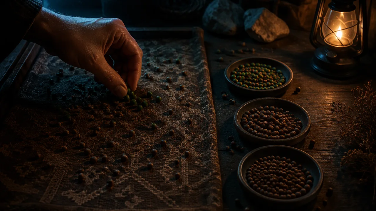
Measuring change with proportions. 9-12.LS4.B.2 asks you to use statistics to show that an advantageous trait increases in proportion. Proportions matter because a population’s size can rise and fall while the fraction with a trait steadily changes. Today’s model: 50 green dots and 50 brown dots (the prey) are scattered on brown patterned fabric (the habitat). “Predators” pick up as many dots as they can in 20 seconds. Survivors reproduce: each survivor is replaced by itself plus offspring of the same color until the population is back to 100. The model has a real Missouri counterpart: banded sculpins, mottled brown fish that MDC describes as well camouflaged by their pattern of light and dark among the rocks of Ozark stream bottoms.
An illustrative run. Suppose predators remove 60% of the green dots and 20% of the brown dots each round. Generation 1: 50 green, 50 brown, proportion brown 0.50. Survivors: 20 green, 40 brown, 60 in all. Scaling back to 100: 33 green and 67 brown, proportion brown 0.67. Repeating: generation 3 has 20 green and 80 brown (0.80), and generation 4 has 11 green and 89 brown (0.89). The brown trait did not appear because it was needed; it was already present, and it was passed on more often because brown dots were harder to see.
Is the change more than chance? Any single round could favor one color by luck. Two habits protect against being fooled. First, repeat the run: if brown increases in every one of several independent runs, chance is an unlikely explanation. Second, compare with a control habitat where neither color is camouflaged, such as white paper; there, you expect proportions to wander around 0.5 with no steady trend. A steady trend in the camouflaged habitat and no trend in the control is strong evidence of selection.
A small advantage adds up. The advantage need not be large. In a simple model where carriers of a trait leave 25% more surviving offspring than non-carriers (equivalently, non-carriers leave 20% fewer), a trait starting at 10% of a population rises to about 51% in 10 generations: 0.10, 0.12, 0.15, 0.18, 0.21, 0.25, 0.30, 0.35, 0.40, 0.45, 0.51. Over the thousands of generations in the history of a population like Missouri’s cave fish, small advantages can produce large differences.
📖 Read for this lesson
The reading opens over the lesson; close it to come back to exactly where you were. The checks below draw on it.
Lab: Camouflage and predation: selection on colored dots
Question. Does the proportion of a camouflaged prey color increase over generations when predators hunt by sight?
Materials
- A patterned brown towel, blanket or piece of fabric about 1 m × 1 m (the habitat) and a plain white sheet, pillowcase or several sheets of white paper (the control habitat)
- Paper dots in two colors, at least 200 of each, punched with a hole punch from brown paper (a paper bag works) and green paper
- A timer (a phone works), small cups, and a data sheet or spreadsheet
- Hole punches can pinch fingers; punch the dots before the lab, with an adult’s help if needed.
- Pick up dots with fingers or tweezers only, and move carefully around the fabric to avoid tripping; keep the floor clear.
Procedure
- Scatter 50 brown and 50 green dots evenly over the patterned fabric without looking where they land (or have a family member scatter them while you look away).
- Hunt as the predator: for 20 seconds, pick up dots one at a time and drop them in a cup. Take three 20-second turns (family members may take a turn each instead). Count the dots of each color that survive on the fabric.
- Reproduction: for each surviving dot, add dots of the same color so that the population returns to 100, keeping the colors in the same proportion as the survivors (round to whole dots). Record the new counts.
- Repeat for four generations, recording the number and proportion of each color each time.
- Repeat the whole experiment on the white control habitat.
- If you can, run each habitat a second time. Set your runs beside the six-run record in the reading and graph the proportion of brown dots against generation for both habitats.
Data
| Generation | Brown at start | Green at start | Proportion brown | Brown survivors | Green survivors |
|---|---|---|---|---|---|
| 1 | 50 | 50 | 0.50 | ||
| 2 | |||||
| 3 | |||||
| 4 |
Analysis
- Describe the trend in the proportion of brown dots in each habitat. Use your own runs and the six-run record in the reading, and state the change from generation 1 to generation 4.
- Map each of the four factors of natural selection (9-12.LS4.B.1) onto a part of the model.
- Why does the control habitat matter to your claim? What result there would weaken it?
- Identify two ways the model differs from real predation or inheritance (for example, all offspring exactly like the parent) and how each might change the result.
If you cannot do this lab in person: Run the PhET Natural Selection simulation with wolves on, brown fur added, in the arctic environment, and record the proportion of brown bunnies each generation; or use the six-run record in the reading together with the illustrative run in the lesson.
Formative check
Work through these before moving on. They are not graded — they tell you whether the standard below has landed yet.
After predation, 20 green and 40 brown dots survive. Scaled back to 100, there are about brown dots, a proportion of .
Which is NOT one of the four factors in 9-12.LS4.B.1?
A steady rise in the proportion of a trait across many independent runs and generations, with no rise in a control habitat, is evidence that selection rather than chance is at work.
A population drops from 1,000 to 600 but the proportion with a camouflage trait rises from 0.30 to 0.45. What does this show?
How confident are you that you can use proportions from a selection model to show that an advantageous trait increases?
Practice
Work these on paper or in your notebook, then open Check your answer. Aim for all of Fluency and Application; try at least one Challenge.
Printable version: this unit’s practice workbook (PDF)
Fluency
Build speed and accuracy with the core skill.
- A population has 33 green and 67 brown dots. What proportion is brown?
Check your answer
Answer: 0.6767 ÷ 100. - After predation, 8 green and 64 brown dots survive. Scale back to 100 and give the new proportion of brown.
Check your answer
Answer: About 11 green and 89 brown; proportion brown 0.89Total 72; 64/72 = 0.889. - List the four factors of natural selection in 9-12.LS4.B.1.
Check your answer
Answer: Potential to increase in number; heritable variation; competition for limited resources (and other threats); proliferation of individuals better able to survive and reproduceAll four are needed together.
Application
Use the skill in context. Show your reasoning.
- Start with 50 green and 50 brown dots. Predators remove 60% of green and 20% of brown each round, and the population is scaled back to 100. Find the proportion of brown after one round.
Check your answer
Answer: About 0.67Survivors: 20 green, 40 brown. 40 ÷ 60 = 0.667. - A trait starts at 10% of a population. Carriers leave offspring at full rate and non-carriers at 80% of that rate. Find the trait’s frequency after one, two and three generations.
Check your answer
Answer: About 0.122, 0.148 and 0.178q′ = q ÷ (q + 0.8(1 − q)): 0.1/0.82 = 0.122; 0.122/0.8244 = 0.148; 0.148/0.8296 = 0.178. - In eight repeated runs, the brown proportion rose in all eight on the patterned fabric, but rose in four and fell in four on white paper. What do these results show?
Check your answer
Answer: On the patterned fabric the consistent rise across replicates is evidence of selection for camouflage. On white paper there is no consistent trend, so changes there are consistent with chance; the control supports the claim that background color caused the difference.Replication plus a control separate selection from chance.
Challenge
Stretch problems. Expect to think before you write.
- A trait starts at 5% of a population and carriers leave twice as many offspring as non-carriers. Find its frequency after each of five generations, and explain why the increase is slow at first and then fast.
Check your answer
Answer: 0.095, 0.174, 0.296, 0.457, 0.627. When the trait is rare, few individuals carry it, so even a large advantage adds few new carriers; as it becomes common, each generation adds many more.q′ = q ÷ (q + 0.5(1 − q)) applied five times from 0.05.
Review
Keep earlier skills sharp.
- For the data 3, 8, 11, 13, 27, 28, 30, 34: find the mean, median, range and interquartile range. (Find the quartiles as the medians of the lower and upper halves, leaving out the overall median when the count is odd.)
Check your answer
Answer: mean = 19.25; median = 20.0; range = 31; IQR = 19.5 (Q1 = 9.5, Q3 = 29.0)
Six Runs, Two Habitats, Four Generations: A Full Record for the Dot Hunt
SLS illustrative data set for the camouflage-and-predation investigation (constructed teaching data, not measurements), with the lesson’s deterministic run and the small-advantage model worked out · SLS original
Why this reading. The analysis asks you to describe the trend using your own runs together with this record, and to say what result in the control habitat would weaken your claim. One run at home is a small sample, and a single run can be swayed by luck. Here is a full illustrative record: six independent runs, four generations, both habitats. These are constructed teaching data, not measurements. If you ran the lab, set your own numbers beside these and compare.
Procedure summarized
Each run scattered 50 brown and 50 green paper dots on a 1 m square of brown patterned fabric. The predator had three 20-second turns to pick up dots one at a time. Survivors of each color were counted and the population was rebuilt to 100 in the survivors’ proportions (rounded to whole dots). Four generations. The whole run was repeated on plain white paper as the control habitat.
Patterned habitat: proportion of brown dots at the start of each generation
| Run | Gen 1 | Gen 2 | Gen 3 | Gen 4 | Gen 5 (after 4 rounds) |
|---|---|---|---|---|---|
| A | 0.50 | 0.64 | 0.77 | 0.86 | 0.92 |
| B | 0.50 | 0.69 | 0.83 | 0.90 | 0.95 |
| C | 0.50 | 0.61 | 0.72 | 0.84 | 0.90 |
| D | 0.50 | 0.67 | 0.80 | 0.89 | 0.94 |
| E | 0.50 | 0.58 | 0.75 | 0.85 | 0.91 |
| F | 0.50 | 0.70 | 0.81 | 0.88 | 0.93 |
| Pooled mean | 0.50 | 0.65 | 0.78 | 0.87 | 0.93 |
Run A’s survivor counts, so you can see the arithmetic: round 1, 21 green and 38 brown survived (59), rebuilt to 36 green and 64 brown; round 2, 15 green and 49 brown (64), rebuilt to 23 and 77; round 3, 9 green and 55 brown, rebuilt to 14 and 86; round 4, 5 green and 61 brown, rebuilt to 8 and 92.
Control habitat (white paper): proportion of brown dots
| Run | Gen 1 | Gen 2 | Gen 3 | Gen 4 | Gen 5 |
|---|---|---|---|---|---|
| A | 0.50 | 0.53 | 0.49 | 0.52 | 0.50 |
| B | 0.50 | 0.47 | 0.45 | 0.48 | 0.46 |
| C | 0.50 | 0.52 | 0.55 | 0.53 | 0.56 |
| D | 0.50 | 0.49 | 0.51 | 0.47 | 0.49 |
| E | 0.50 | 0.46 | 0.48 | 0.50 | 0.47 |
| F | 0.50 | 0.54 | 0.52 | 0.55 | 0.53 |
| Pooled mean | 0.50 | 0.50 | 0.50 | 0.51 | 0.50 |
What the two tables show
On the patterned fabric every one of six runs rose every generation, from 0.50 to between 0.90 and 0.95 after four rounds: a change of about +0.43 in the pooled proportion. On white paper the six runs wandered between 0.45 and 0.56 with no direction, and the pooled mean stayed at 0.50. A rise in one run could be luck; a rise in six of six, with the same dots and the same predators producing no rise on white paper, is not. That is the logic of the true-or-false check: replication rules out chance, and the control rules out every explanation that does not involve the background.
The result that would weaken the claim is a rise in brown on the white paper too. It would mean predators were picking green for some reason other than visibility, such as a color preference, or that the reproduction step was biased. The control’s flat line is what lets you say the background did the selecting.
The lesson’s deterministic run, reproduced
If predators removed exactly 60 percent of green and 20 percent of brown every round: generation 1, 50/50 (0.50); survivors 20 green and 40 brown, rebuilt to 33 and 67 (0.67); survivors 13.2 and 53.6, rebuilt to 20 and 80 (0.80); survivors 8 and 64, rebuilt to 11 and 89 (0.89). The six-run record above lands in the same place by a noisier road, which is what real predators do.
The small-advantage model, reproduced
If carriers of a trait leave 1.25 offspring for every 1.00 left by non-carriers, the proportion p becomes 1.25p ÷ (1.25p + (1 − p)) each generation. From 0.10: 0.12, 0.15, 0.18, 0.21, 0.25, 0.30, 0.35, 0.40, 0.45, 0.51 after ten generations, exactly the sequence in the lesson. Continue it and the trait passes 0.90 by about generation 20. A cave fish such as the Ozark cavefish can live 10 years or more; twenty of its generations outlast a human lifetime, and Missouri’s cave fish lineages have had far more than that.
Mapping the four factors onto the model
| Factor (9-12.LS4.B.1) | Where it is in the model |
|---|---|
| Potential to increase in number | Every round rebuilds the population to 100: survivors more than replace themselves |
| Heritable variation | Two colors, and every offspring dot is the same color as its parent |
| Competition and limited survival | Predators remove about 40 percent of dots every round; the population cannot exceed 100 |
| Traits suited to the environment leave more offspring | Brown dots on brown fabric survive predation more often, so their share of the rebuilt population grows |
Two ways the model is unlike life
- Offspring are identical to parents; real inheritance mixes two parents and produces intermediate colors, which slows the change.
- Predators hunt only by sight, only for 20 seconds, with no learning; real predators learn search images, which can strengthen selection against a common prey and weaken it against a rare one.