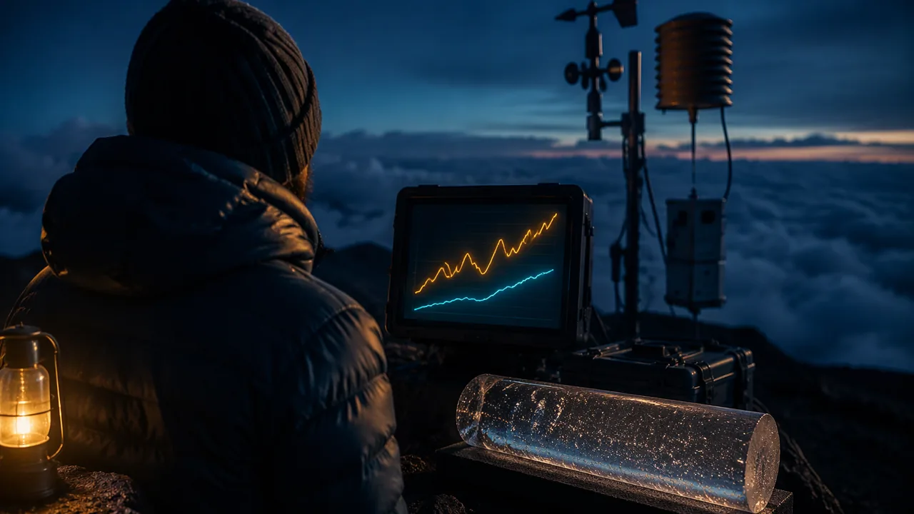
analyze the Mauna Loa carbon dioxide record and the NASA global temperature record, calculate rates of change for different periods, and ask questions about what the patterns mean.
Instruction
The phenomenon. In 1958 the scientist Charles David Keeling began measuring carbon dioxide on Mauna Loa, a volcano in Hawaiʻi whose summit sits high above local pollution and forests. NOAA and the Scripps Institution of Oceanography have continued the record ever since. The annual mean was 315.98 parts per million (ppm) in 1959, 369.71 ppm in 2000, and 424.61 ppm in 2024. Air bubbles trapped in Antarctic ice show that for at least 800,000 years before industrialization, carbon dioxide stayed between about 180 and 300 ppm, and it was about 280 ppm in the 1700s.
Two patterns in one curve. The Keeling curve rises every year, and it also wiggles: each year carbon dioxide falls by about 6 ppm from May to late September and rises again through winter. The wiggle is the Northern Hemisphere’s plants breathing: in summer, photosynthesis draws carbon dioxide out of the air; in winter, decay and respiration return it. The biosphere and atmosphere exchange carbon every year. The rise underneath is something else.
Worked example: rates of change. A rate is change divided by time. From 1959 to 1969 the annual mean rose 0.86 ppm per year on average. From 2014 (398.81 ppm) to 2024 (424.61 ppm) it rose (424.61 − 398.81) / 10 = 2.58 ppm per year, three times as fast. The total rise since 1959 is 108.63 ppm, 34%. Compared with 280 ppm, the 2024 level is about 52% higher. When the rate itself is increasing, the curve bends upward, and a straight-line forecast will underestimate the future unless something changes.
Temperature. NASA’s GISTEMP analysis combines thousands of weather stations and ocean measurements into a global average, reported as an anomaly: the difference from the 1951-1980 average. The mean anomaly for 1880-1899 was about −0.22 °C. In 2024 it was 1.28 °C, the warmest year in the record, about 1.5 °C above the late 1800s; 2025 (1.18 °C) was second. Single years jump up and down with El Niño and La Niña, so scientists look at trends: a least-squares line through 1975-2024 rises about 0.20 °C per decade. Averaged over 2015-2024, the world was about 1.2 °C warmer than in 1880-1899.
Reading the data honestly. Two records rising together do not by themselves prove that one causes the other. The case for cause comes from physics (Unit 2: carbon dioxide absorbs infrared energy), from fingerprints, and from models, which you will examine in this unit. Good questions separate what the data show from what they mean: How much of the carbon dioxide comes from fossil fuels, and how do we know? Where does the rest of the carbon go? Is Missouri warming as fast as the globe?
Closer to home. NOAA’s National Centers for Environmental Information keep a statewide temperature record for Missouri back to 1895. Its three warmest years are 2012 (58.6 °F), 2024 (57.9 °F) and 1921 (57.6 °F). A least-squares line through the whole record, 1895-2025, rises only about 0.10 °F per decade, because the 1930s Dust Bowl years were very hot and the 1960s and 1970s cool. A line through 1975-2025 rises about 0.50 °F (0.28 °C) per decade, faster than the global average, as you would expect for the middle of a continent. Same data, two honest answers: the period you choose changes the rate, so always name it. NOAA’s State Climate Summary for Missouri adds that the warming has come mostly in winter, spring and summer nights, while summer daytime highs have not risen much.
Scale. Keep units straight: 1 ppm of carbon dioxide in the whole atmosphere contains about 2.13 billion metric tons (gigatons) of carbon. The 2024 level, 424.61 ppm, is about 904 gigatons of carbon in the air.
📖 Read for this lesson
The reading opens over the lesson; close it to come back to exactly where you were. The checks below draw on it.
Formative check
Work through these before moving on. They are not graded — they tell you whether the standard below has landed yet.
Simulation & tools
Global temperature, your way
Open NOAA’s Climate at a Glance global time series. Choose Globe, Land and Ocean, 12-Month (annual), all years. Turn on the trend line and set it to start in 1975. Record the trend NOAA reports per decade and the three warmest years. Compare them with the NASA figures in this lesson: do two independent analyses agree? Then switch to the Statewide view, choose Missouri, Average Temperature, 12-Month, and record the trend from 1895 and from 1975. Is Missouri warming faster or slower than the globe, and why does the start year matter so much?
No device? Use the GISTEMP table in the reading rlp-esb-keeling-curve-context and the Missouri tables in rlp-esb-missouri-climate-record to find the warmest years and compute rates from 1975 to 2024 by hand.
Open NOAA ↗ · NOAA · Public domain (U.S. federal)
From 2014 (398.81 ppm) to 2024 (424.61 ppm), carbon dioxide rose about ppm per year, about times the rate of the 1960s (0.86 ppm per year).
What causes the yearly up-and-down wiggle in the Keeling curve?
Because 2025 was cooler than 2024 in the NASA record, global warming stopped in 2025.
Sketch the Keeling curve and the GISTEMP record on one page and annotate three features (the wiggle, the steepening rise, the El Niño years). Then write two investigable questions: one about where the added carbon dioxide comes from, and one about what the trend means for Missouri.
How confident are you that you can analyze long climate records and calculate rates of change for different periods?
Practice
Work these on paper or in your notebook, then open Check your answer. Aim for all of Fluency and Application; try at least one Challenge.
Printable version: this unit’s practice workbook (PDF)
Fluency
Build speed and accuracy with the core skill.
- Use technology to find the least-squares line and the correlation coefficient for (1, 10), (2, 13), (10, 33), (12, 35), (13, 39).
Check your answer
Answer: ŷ = 8.059 + 2.361x; r = 0.997Interpret the slope in context: the predicted change in y for each one-unit increase in x. - Mauna Loa CO2 was 369.71 ppm in 2000 and 390.10 ppm in 2010. What was the average rate?
Check your answer
Answer: 2.04 ppm per year - It was 390.10 ppm in 2010 and 414.21 ppm in 2020. What was the average rate?
Check your answer
Answer: 2.41 ppm per year - By what percentage is 424.61 ppm (2024) above the pre-industrial 280 ppm?
Check your answer
Answer: about 52%
Application
Use the skill in context. Show your reasoning.
- NASA GISTEMP anomalies (relative to 1951-1980) were −0.02 °C in 1960, 0.26 in 1980, 0.39 in 2000 and 1.01 in 2020. Compute the change per decade for 1960-1980 and 2000-2020.
Check your answer
Answer: 1960-1980: 0.14 °C per decade; 2000-2020: 0.31 °C per decadeChange divided by two decades. - The 1880-1899 mean anomaly was about −0.22 °C and 2024 was 1.28 °C. How much warmer was 2024 than the late 1800s?
Check your answer
Answer: about 1.5 °C - At 1 ppm = 2.13 GtC, how many gigatons of carbon did the atmosphere gain from 2014 (398.81 ppm) to 2024 (424.61 ppm)?
Check your answer
Answer: about 55 GtC
Challenge
Stretch problems. Expect to think before you write.
- A least-squares line through 1975-2024 GISTEMP rises about 0.20 °C per decade and gives an anomaly of about 1.54 °C in 2050. Explain why this straight-line forecast could be too low or too high, giving one reason each way.
Check your answer
Answer: Too low if warming accelerates as emissions continue and feedbacks grow; too high if emissions fall quickly. A trend line assumes the causes of the past continue unchanged.
Review
Keep earlier skills sharp.
- Review (Unit 2): find the CO2 forcing at 400 ppm using 5.35 ln(C/280).
Check your answer
Answer: about 1.91 W/m2
Charles Keeling’s Curve, and the Temperature Record Beside It
NOAA Global Monitoring Laboratory, co2_annmean_mlo.txt, and NASA GISS GISTEMP v4, GLB.Ts+dSST.csv (both public domain), retrieved November 6, 2026 · Public domain (works of the United States government), with SLS original arithmetic and framing
Why this reading. The lesson’s mini-lecture states the Keeling and GISTEMP numbers you need for the fill-in-the-blank and the sim task. This reading gives the table behind those numbers and the story of why Charles Keeling’s measurement method still matters. Open the companion reading rlp-alg2b-mauna-loa-co2-record beside it: its Table 1 is the Mauna Loa annual-mean record from 1959 to 2025 (skip its exponential-model sections). For Missouri’s own temperature record, use rlp-esb-missouri-climate-record.
Why Mauna Loa, and why it took discipline to trust it
Charles David Keeling began continuous carbon dioxide measurements at the Mauna Loa Observatory in Hawaiʻi (elevation 3,397 m) in March 1958, during the International Geophysical Year. He chose the site because its air, high above local vegetation, traffic and industry, samples the well-mixed background atmosphere rather than a city’s exhaust or a forest’s daily breathing. Keeling insisted on a calibration standard precise enough to see year-to-year change, at a time when many scientists doubted that carbon dioxide could be measured reliably at all. NOAA’s Global Monitoring Laboratory and the Scripps Institution of Oceanography have run parallel programs at the observatory since 1974, so a second, independent instrument checks the first.
The isotopic preview
One question this lesson asks you to raise — where does the added carbon dioxide come from? — is answered with a specific kind of evidence: the proportion of the heavier carbon isotope, carbon-13, in atmospheric CO2 has been falling as CO2 has risen, because carbon from ancient plants (coal, oil and gas) is isotopically lighter. This is the “isotopic fingerprint” the glossary in Lesson 3.3 names. Hold the question until then.
Table 1. NASA GISTEMP global temperature anomaly, selected years (°C, relative to the 1951–1980 average)
| Period / year | Anomaly (°C) | Note |
|---|---|---|
| 1880–1899 average | −0.22 | Late-1800s baseline the lesson cites |
| 1960 | −0.02 | |
| 1975 | −0.01 | Start year of the lesson’s trend line |
| 1980 | 0.26 | |
| 2000 | 0.39 | |
| 2014 | 0.75 | Warmest year on record at the time |
| 2016 | 1.01 | Strong El Niño year |
| 2020 | 1.01 | Tied 2016 without a strong El Niño |
| 2023 | 1.17 | |
| 2024 | 1.28 | Warmest year on record |
| 2025 | 1.18 | Second-warmest |
GISTEMP is revised slightly as late station reports arrive, so a figure printed a year ago can differ by 0.01 °C from today’s file. These values are from the file as retrieved on November 6, 2026.
Reading the table. Single years do not move smoothly: 2016 and 2020 are tied even though 2016 rode a strong El Niño (a natural warming pulse in the tropical Pacific) and 2020 did not. That is why “2025 was cooler than 2024, so warming stopped” is false: a one-year dip inside a rising trend is ordinary. Second, the gap between 1975 (−0.01) and 2024 (1.28) is 1.29 °C over 49 years, about 0.26 °C per decade on the endpoints alone. A least-squares line through every year from 1975 to 2024, the lesson’s “about 0.20 °C per decade” (SLS fit: 0.203), is lower because no single year at either end pulls it around. Extended to 2050, that line reaches an anomaly of about 1.54 °C. Endpoint rate versus least-squares rate is a distinction your Lesson 3.5 forecast must make explicit.
Two more checks. 2024 minus the 1880–1899 average is 1.28 − (−0.22) = 1.50 °C. The 2015–2024 average anomaly is 0.98 °C, which is 1.21 °C above the 1880–1899 average: “about 1.2 °C warmer” in the lesson.
Reading NOAA’s own trend tool
The lesson’s sim task sends you to NOAA’s Climate at a Glance, which uses NOAA’s own analysis (NOAAGlobalTemp) rather than NASA’s GISTEMP. The two agencies’ values for one year can differ by a few hundredths of a degree because they treat sparse Arctic and ocean coverage differently, but their decade-scale trends agree closely: independent groups, independent methods, the same answer. The same tool also holds every U.S. state’s record, including Missouri’s.
Scale, restated
1 ppm of atmospheric carbon dioxide is about 2.13 gigatons of carbon (GtC). From 2014 (398.81 ppm) to 2024 (424.61 ppm) the air gained 25.80 ppm, or 25.80 × 2.13 ≈ 55 GtC. Keep the units and the years attached to every number you write down; a rate with no stated period is not a rate you can defend.
Sources: NOAA GML, annual mean CO2 at Mauna Loa (data file) (gml.noaa.gov); NASA GISS, GISTEMP v4 global land-ocean annual means (data file) (data.giss.nasa.gov); NOAA NCEI Climate at a Glance, global time series (ncei.noaa.gov)
Sixty-Six Years of Carbon Dioxide: A Record That Almost Fits an Exponential
NOAA GML, annual mean carbon dioxide at Mauna Loa Observatory, file co2_annmean_mlo.txt (created October 9, 2026), retrieved November 5, 2026 · Public domain (works of the United States government)
Why this reading. The workshop asks you to solve abct = d for real, and to derive and interpret an inverse. Solving for t is only interesting when someone actually wants the answer to “when?” This is the longest continuous record of atmospheric carbon dioxide in the world, from NOAA’s Mauna Loa Observatory. Values are annual means in parts per million, dry air mole fraction.
Table 1. Annual mean CO2, Mauna Loa (ppm)
| Year | 1959 | 1960 | 1970 | 1980 | 1990 | 2000 | 2005 |
|---|---|---|---|---|---|---|---|
| ppm | 315.98 | 316.91 | 325.68 | 338.76 | 354.45 | 369.71 | 379.98 |
| Year | 2010 | 2015 | 2020 | 2021 | 2022 | 2023 | 2024 |
| ppm | 390.10 | 401.01 | 414.21 | 416.41 | 418.53 | 421.08 | 424.61 |
| Year | 2025 | The full file carries every year from 1959 to 2025, with a stated uncertainty of 0.12 ppm. | |||||
| ppm | 427.35 | ||||||
Three models, three answers to the same question
Let t be years after 1960 and C(t) the annual mean. Take 450 ppm as the level to solve for — a round number, and one that appears in policy discussion.
Model A, the endpoints 1960 and 2025. The growth factor is (427.35/316.91)1/65 = 1.004610, so CA(t) = 316.91(1.004610)t, about 0.461% a year. Solve 316.91(1.004610)t = 450: t = ln(450/316.91) / ln 1.004610 = 76.2, which lands in 2036. Check the model in the middle: CA(30) = 363.8 against an actual 354.45 in 1990. It is 9.4 ppm high, and always high in the middle, because the early years grew more slowly than the endpoints imply.
Model B, a least-squares fit to all 66 years. Regressing ln C on t gives a factor of 1.004641, about 0.464% a year, with 1960 value 310.15. Solving for 450 from the 2025 value gives 11.2 years, so again about 2036. The two exponential models agree almost exactly on the date and still both miss: this model predicts 419.05 for 2025 against an actual 427.35.
Model C, the last twenty years. (427.35/379.98)1/20 = 1.005892, about 0.589% a year. Solving ln(450/427.35)/ln 1.005892 = 8.8 years puts 450 ppm in 2034.
A linear model, for comparison. Least squares on the raw ppm gives 1.686 ppm a year, reaching 450 in 2045. That is nine to eleven years later than any of the exponential models, and the reason is visible in the data: the gaps between decades are 8.8, 13.1, 15.7, 15.3, 20.4 and 24.1 ppm. The increments themselves are growing, so a constant-slope line will always fall behind. Exponential is the better shape here, even though none of these models is a physical theory of anything.
The inverse, and what it is for
Model A’s inverse answers “what year?” directly. From C = 316.91(1.004610)t, solve for t: t(C) = ln(C/316.91) / ln 1.004610, defined for C > 0, and meaningful for C above 316.91, the range of CA on t ≥ 0. The composition check is the whole point of an inverse: t(CA(65)) should return 65, and it does. Doubling time, from ln 2 / ln 1.004610, is 150.7 years — a number worth saying out loud, because it shows how slow 0.46% a year sounds and how fast 111 ppm in 66 years looks.
Where the model is wrong, and why that matters
Annual means hide a sawtooth. Mauna Loa readings rise and fall within every year by about 6 ppm as Northern Hemisphere plants take up carbon in summer and release it in autumn — the seasonal signal you will model with a sinusoid in Unit 3. An annual-mean model cannot tell you the value in May. More importantly, no exponential is a mechanism. This curve bends because of emissions, oceans and land uptake, all of which are policy- and physics-dependent, and any of which can change the curve inside a decade. A model that tells you 2036 is telling you what the last sixty-six years would give if nothing changed. Report the date and that sentence, or you have not reported the model.
Two more to solve. When does Model C reach 500 ppm? When did Model A pass 400 ppm, and how does that compare with the year the record actually crossed it? Both are one logarithm each, and both are worth checking against Table 1 rather than trusting.
Sources: NOAA Global Monitoring Laboratory, Trends in atmospheric carbon dioxide (gml.noaa.gov); NOAA GML, annual mean CO2 at Mauna Loa (data file) (gml.noaa.gov)
Missouri’s Own Climate Record: 131 Years of Statewide Temperature
NOAA NCEI Climate at a Glance, Missouri statewide annual average temperature 1895-2025 (data.csv); NOAA NCEI State Climate Summaries 2025, Missouri; both retrieved November 6, 2026 · Public domain (works of the United States government), with SLS original arithmetic
Why this reading. A global average is not where anyone lives. This reading hosts Missouri’s statewide temperature record from NOAA’s National Centers for Environmental Information (NCEI) and the main findings of NOAA’s State Climate Summary for Missouri, so you can compute Missouri rates for different periods (Lesson 3.1) and build the Missouri part of your forecast (Lesson 3.5). Temperatures are in °F, as NOAA publishes them; a change of 1 °F equals 5/9 °C, about 0.56 °C.
Table 1. Missouri statewide average temperature, decade means (°F)
| Decade | 1900s | 1910s | 1920s | 1930s | 1940s | 1950s | 1960s |
|---|---|---|---|---|---|---|---|
| Mean | 54.03 | 54.25 | 54.51 | 55.71 | 54.56 | 54.70 | 53.89 |
| Decade | 1970s | 1980s | 1990s | 2000s | 2010s | 2020–2025 | |
| Mean | 54.00 | 54.46 | 54.89 | 55.24 | 55.65 | 56.48 |
Table 2. Selected years (°F)
| Year | 1921 | 1934 | 1975 | 2012 | 2021 | 2022 | 2023 | 2024 | 2025 |
|---|---|---|---|---|---|---|---|---|---|
| °F | 57.6 | 56.6 | 54.6 | 58.6 | 56.3 | 55.0 | 57.4 | 57.9 | 56.5 |
The three warmest years in the record are 2012 (58.6 °F), 2024 (57.9 °F) and 1921 (57.6 °F). The 1895–2024 average is 54.7 °F, so 2012 was 3.9 °F above it, the figure the State Climate Summary reports.
Table 3. Missouri rates depend on the period you choose (SLS least-squares fits to the NCEI annual values)
| Fitting period | Trend (°F per decade) | Trend (°C per decade) | Line extended to 2050 (°F) |
|---|---|---|---|
| 1895–2025 (whole record) | 0.10 | 0.055 | 55.6 |
| 1950–2025 | 0.28 | 0.15 | 56.6 |
| 1975–2025 | 0.50 | 0.28 | 57.6 |
Over the whole record the line rises about 0.10 °F per decade, about 1.3 °F in total: the State Climate Summary’s “more than 1°F since the beginning of the 20th century.” Since 1975 the rate is five times faster, 0.50 °F (0.28 °C) per decade, faster than the global 0.20 °C per decade, as expected for the interior of a continent (land warms faster than ocean). Why so different? The 1930s Dust Bowl decade was very hot in Missouri, and the 1960s and 1970s were cool, so a line that starts in 1895 is flattened by that hump and dip. Neither number is wrong; each answers a different question, and a forecast must say which period it used and why. Comparing averages: 2016–2025 averaged 56.37 °F, which is 1.78 °F (about 1.0 °C) warmer than the 1901–1960 average of 54.59 °F.
What NOAA’s State Climate Summary for Missouri reports
- Where the warming is. Warming has been concentrated in winter and spring; summers have not warmed substantially. Summer daytime highs have been near or below the long-term average since the late 1980s, and the hottest summers on record are still those of the 1930s Dust Bowl. Summer nights have warmed: at St. Louis Lambert International Airport, very warm nights (75 °F or higher) rose from 13 per year in 1961–1990 to 20 per year in 1991–2024. Very cold nights (0 °F or lower) have been below average since the 1990s.
- Rain. Statewide annual precipitation averages 41.1 inches and has generally been near or above average since the 1990s. Missouri has had a near- or above-average number of 2-inch downpours since the 1980s (long-term average 2.3 such days per year at a typical station).
- Projections. Under intermediate and higher emissions, historically unprecedented warming is projected this century. The summary’s figure shows end-of-century Missouri warming relative to 1901–1960 of about 1.9–8.2 °F under lower emissions (SSP1-2.6), 4.2–11.0 °F under intermediate emissions (SSP2-4.5) and 8.4–17.7 °F under higher emissions (SSP5-8.5). Extreme precipitation is projected to become more frequent and intense, raising flood risk in a state that sits in the lower basins of several large rivers; rising temperatures are projected to make droughts more intense. Projected changes in total annual precipitation are small and not statistically significant.
Try it. (1) Compute the endpoint rate from 1975 (54.6 °F) to 2024 (57.9 °F) and compare it with the least-squares 0.50 °F per decade. (2) Explain, using Table 1, why a Missouri trend computed from 1930 to 1970 would show cooling. (3) Convert 0.50 °F per decade to °C per decade.
Sources: NOAA NCEI Climate at a Glance, Missouri statewide January-December average temperature, 1895-2025 (data file) (ncei.noaa.gov); NOAA NCEI / NCICS, State Climate Summaries 2025: Missouri (statesummaries.ncics.org)