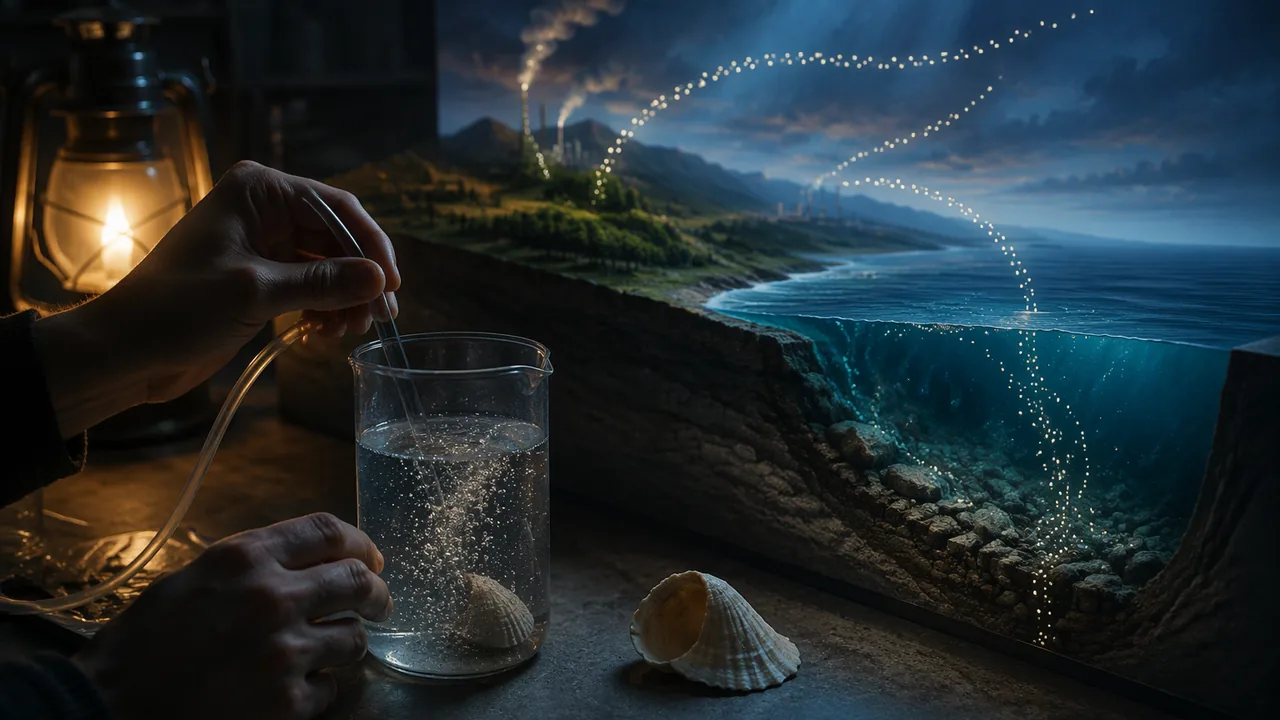
investigate how carbon dioxide dissolves in water, acidifies it and dissolves carbonate shells, and use a quantitative model of carbon reservoirs and flows to explain where emitted carbon goes.
Instruction
Carbon moves. Carbon is stored in reservoirs and moves between them in fluxes. A quantitative model of the carbon cycle tracks both, in gigatons of carbon (GtC). Approximate reservoir sizes, from the Global Carbon Budget and the IPCC’s assessments: the atmosphere about 900 GtC; living plants about 450 GtC and soils well over 1,500 GtC; the ocean about 38,000 GtC, most of it dissolved in deep water; and sedimentary rocks such as limestone tens of millions of GtC, by far the largest store. Fossil fuels are a small part of the rock reservoir: carbon that plants and plankton stored over millions of years.
Fast and slow cycles. Every year, photosynthesis and respiration move on the order of a hundred GtC in and out of the atmosphere, and the ocean surface exchanges a similar amount. Those fast flows nearly balance. The slow cycle, in which carbon moves into and out of rocks by weathering, burial, subduction and volcanoes, takes hundreds of thousands to millions of years (Earth Science A, Unit 4). Burning fossil fuels short-circuits the slow cycle: it moves rock carbon into the air in decades.
Worked example: where does our carbon go? In recent years, fossil fuels and cement released about 10 GtC per year and land-use change (mostly deforestation) roughly 1 more, about 11 GtC in all. Over 2014-2024 the atmosphere gained 2.58 ppm per year, and 2.58 × 2.13 ≈ 5.5 GtC. So 5.5 / 11 ≈ 50% of emissions stayed in the air: this is the airborne fraction. The rest, roughly half, was taken up in about equal shares by the ocean and by land plants and soils. The ocean and land are doing us a favor, but not for free.
The ocean’s chemistry. Carbon dioxide dissolves in seawater and forms carbonic acid: CO2 + H2O → H2CO3, which releases hydrogen ions. More hydrogen ions mean lower pH. The pH scale is logarithmic: a drop of 1 unit means 10 times the hydrogen-ion concentration. Surface ocean pH has fallen by about 0.1 since pre-industrial times, and 100.1 ≈ 1.26, a rise of about 26% in hydrogen ions (often reported as about 30%, since the drop is slightly more than 0.1). This is ocean acidification. The extra hydrogen ions also use up carbonate ions that corals, oysters, sea urchins and tiny plankton need to build calcium carbonate shells. Along the Pacific Northwest coast, upwelled water is naturally rich in carbon dioxide, so acidification adds to an existing stress: an Oregon oyster hatchery lost 70 to 80 percent of its larvae from 2006 to 2008 when corrosive water reached them. Missouri has no coast, but its rocks record the same chemistry running the other way: the Burlington Limestone, found throughout the state, is packed with fossil crinoids, Missouri’s state fossil, whose calcium carbonate skeletons built up on the floor of a shallow sea in the Mississippian Period, about 360 to 320 million years ago. Shell-building stores carbon in rock; acid water dissolves it.
Temperature and a feedback. Gases dissolve better in cold water. As the ocean warms, it can hold less carbon dioxide, so it takes up a smaller share of emissions: a reinforcing feedback between the hydrosphere and atmosphere. In the lab you will open cold and warm seltzer and compare how much gas escapes.
Your investigation. Seltzer is water with carbon dioxide dissolved under pressure: a model of an ocean absorbing a lot of it. You will measure its pH, test what it does to calcium carbonate (chalk or a shell), and measure how temperature affects how much gas it holds.
📖 Read for this lesson
The reading opens over the lesson; close it to come back to exactly where you were. The checks below draw on it.
Lab: Seltzer, Shells and the Acidifying Ocean
Question. How does dissolved carbon dioxide change the pH of water and the rate at which calcium carbonate dissolves, and how does temperature affect how much carbon dioxide water holds?
Materials
- Two bottles of plain unflavored seltzer (one refrigerated, one at room temperature) and tap water
- pH test strips (range 4-9), or red-cabbage indicator you make with an adult (chop a quarter of a red cabbage, cover with hot tap water, steep 15 minutes, strain)
- Four clear plastic cups, masking tape and a marker
- Plain white chalk or clean seashell or eggshell pieces (calcium carbonate)
- Kitchen scale (0.01 g or 0.1 g) and paper towels
- Two balloons that fit over the bottle necks, a tape measure, and a kitchen thermometer if you have one
- Work with an adult nearby, and wear safety glasses or goggles: seltzer can spray when opened and cabbage indicator can stain or sting eyes.
- Do not drink or taste any lab liquids. Open bottles pointed away from people, wipe up spills at once, and wash hands after the lab.
Procedure
- Pour 100 mL of tap water and 100 mL of room-temperature seltzer into labeled cups. Measure and record the pH of each.
- Weigh two chalk or shell pieces of similar mass. Place one in each cup and observe for 5 minutes, then leave them for 24 hours.
- Next day, remove each piece, blot and air-dry it, weigh it, and compute the percent mass lost. Record the pH of each liquid again.
- Open the cold and the room-temperature seltzer bottles at the same moment and stretch a balloon over each neck at once. Shake each gently for 10 seconds, then measure the circumference of each balloon after 5 minutes.
- Compare which bottle released more carbon dioxide (larger balloon) and record the temperature of each.
Data
| Liquid | pH start | pH after 24 h | Shell/chalk start mass (g) | After 24 h (g) | Mass lost (%) |
|---|---|---|---|---|---|
| Tap water | |||||
| Seltzer |
| Seltzer bottle | Temperature (°C) | Balloon circumference after 5 min (cm) |
|---|---|---|
| Cold | ||
| Room temperature |
Analysis
- Claim: how does dissolved carbon dioxide affect pH and shells? Use your pH readings and percent mass lost as evidence, and explain with the carbonic-acid reaction.
- Did the pH of the seltzer change after 24 hours open to the air? Explain what happened to its carbon dioxide and connect it to the exchange between the ocean surface and the atmosphere.
- Which bottle released more gas? Explain what your result means for how much carbon dioxide a warming ocean can absorb, and identify the feedback.
- Sources of error: how do pH-strip color matching, incomplete drying and differences in shell size affect your results?
If you cannot do this lab in person: If you cannot get pH strips or a scale, place a piece of chalk or eggshell in seltzer and another in tap water and photograph them after 24 hours; or analyze the sample data set in the reading rlp-esb-ocean-carbon-ledger (Table 3) and answer every analysis question from it.
Formative check
Work through these before moving on. They are not graded — they tell you whether the standard below has landed yet.
The atmosphere gains 2.4 ppm of carbon dioxide in a year, and 1 ppm contains 2.13 GtC. If emissions were 11 GtC, what was the airborne fraction?
A drop in ocean pH from 8.2 to 8.1 means about a 26% increase in hydrogen-ion concentration.
Atmosphere
Tap to revealAbout 900 GtC; gains about 5 GtC a year now
Ocean
Tap to revealAbout 38,000 GtC; takes up roughly a quarter of emissions
Plants and soils
Tap to revealAbout 450 GtC in plants and over 1,500 GtC in soils; take up roughly a quarter
Rocks
Tap to revealTens of millions of GtC; the slow cycle, including fossil fuels
Draw a quantitative carbon-cycle model with at least five reservoirs (atmosphere, ocean, plants, soils, rocks and fossil fuels) labeled with their sizes, and arrows for at least five fluxes. Show the human flux (about 11 GtC per year) and where it goes, and mark the feedback you found in the lab.
How confident are you that you can investigate how carbon dioxide affects the ocean and use a quantitative carbon-cycle model to explain where emissions go?
Practice
Work these on paper or in your notebook, then open Check your answer. Aim for all of Fluency and Application; try at least one Challenge.
Printable version: this unit’s practice workbook (PDF)
Fluency
Build speed and accuracy with the core skill.
- How many gigatons of carbon are in the atmosphere at 424.61 ppm (1 ppm = 2.13 GtC)?
Check your answer
Answer: about 904 GtC - The atmosphere gains 2.4 ppm in a year. How many GtC is that?
Check your answer
Answer: about 5.1 GtC - Ocean pH falls from 8.2 to 8.1. By what factor does the hydrogen-ion concentration increase?
Check your answer
Answer: about 1.26 (about 26% more)100.1.
Application
Use the skill in context. Show your reasoning.
- Emissions are 11 GtC per year and the atmosphere gains 2.58 ppm per year. What is the airborne fraction, and where does the rest go?
Check your answer
Answer: about 50%; the rest is taken up by the ocean and by land plants and soils, in roughly equal shares - In the lab a 5.20 g shell piece in seltzer dried to 4.94 g after 24 hours, and one in tap water went from 5.10 g to 5.08 g. Find each percent mass lost and explain the difference.
Check your answer
Answer: seltzer 5.0%; tap water 0.4%; dissolved CO2 forms carbonic acid, which dissolves calcium carbonate - Explain the feedback between ocean temperature and ocean carbon uptake, and say whether it is reinforcing or balancing.
Check your answer
Answer: Warmer water holds less dissolved CO2, so a warming ocean takes up a smaller share of emissions, leaving more in the air and causing more warming: reinforcing.
Challenge
Stretch problems. Expect to think before you write.
- The ocean takes up about a quarter of 11 GtC per year. What fraction of the ocean’s roughly 38,000 GtC reservoir is that each year? Why can this small fraction still change surface-ocean chemistry noticeably?
Check your answer
Answer: about 0.0072% per year; the carbon enters the thin surface layer first and mixes into the deep ocean only over centuries, so the surface changes much faster
Review
Keep earlier skills sharp.
- Review (Unit 2): find the no-greenhouse temperature of a planet absorbing 200 W/m2.
Check your answer
Answer: about 244 K(200 / σ)1/4.
The Ocean’s Carbon Ledger: Reservoirs, the Airborne Fraction, and a Falling pH
Hawaii Ocean Time-series HOT_surface_CO2.txt (updated January 1, 2026); Global Carbon Budget 2025 press release; NOAA NCCOS repost of Yale Environment 360 (2011); IPCC AR6 WGI, cited for its findings; all retrieved November 6, 2026 · SLS original (cites University of Hawaiʻi HOT open data, the Global Carbon Budget, NOAA and IPCC; brief quotations only), with SLS illustrative lab data
Why this reading. The lab asks you to explain the carbonic-acid reaction with real numbers behind it and to connect your balloon result to how much carbon dioxide a warming ocean can absorb. The quiz and true/false items need a published record of ocean pH and a carbon budget to check your airborne-fraction arithmetic. Both are here, plus a sample data set from a home run of the lab for anyone who cannot do it.
Table 1. Station ALOHA (Hawaii Ocean Time-series), surface ocean pH, annual means of the measured cruises
Station ALOHA, about 100 km north of Oʻahu, has been sampled almost monthly since October 1988 by the University of Hawaiʻi’s Hawaii Ocean Time-series. The values below are SLS averages of the in-situ pH (calculated) column in the HOT data file for each year.
| Year | 1989 | 1995 | 2005 | 2015 | 2024 |
|---|---|---|---|---|---|
| Surface pH | 8.11 | 8.10 | 8.08 | 8.07 | 8.04 |
A least-squares line through all 346 cruises from October 1988 to December 2024 falls 0.0019 pH units per year, about 0.02 per decade, from 8.12 to 8.05 on the fitted line: a drop of 0.07. Using the lesson’s rule, 100.07 ≈ 1.18, so hydrogen ions at Station ALOHA rose about 18% in 36 years. Since pre-industrial times, global surface pH has fallen by about 0.1 (8.2 to 8.1), and 100.1 ≈ 1.26, about 26% more hydrogen ions.
Table 2. Global carbon reservoirs and the recent budget (gigatons of carbon, GtC)
| Reservoir or flux | Size or rate | Source |
|---|---|---|
| Atmosphere | ≈904 GtC at 424.61 ppm (2024); gaining about 5.5 GtC a year (2014–2024) | NOAA/Scripps Mauna Loa ppm × 2.13 |
| Fossil fuels + cement, 2025 | 38.1 billion tonnes CO2 = 38.1 × 12/44 ≈ 10.4 GtC | Global Carbon Budget 2025 (projection) |
| Land-use change, 2025 | 4.1 billion tonnes CO2 ≈ 1.1 GtC | Global Carbon Budget 2025 (projection) |
| Total human emission | ≈11 GtC a year (the lesson’s round figure) | sum of the two rows above |
| Ocean store | ≈38,000 GtC | IPCC AR6, cited as a finding |
Multiplying by 12/44 converts a mass of carbon dioxide to the mass of carbon in it (carbon’s atomic mass is 12; CO2‘s molecular mass is 44). Working the lesson’s quiz: a gain of 2.4 ppm is 2.4 × 2.13 ≈ 5.1 GtC; against 11 GtC of emissions, the airborne fraction is 5.1 / 11 ≈ 0.46. For 2014–2024, 2.58 ppm a year is 5.5 GtC, and 5.5 / 11 ≈ 0.50. The remaining half is taken up by the ocean and by land plants and soils in roughly equal shares. The 2025 Global Carbon Budget also reports that climate change is now weakening these land and ocean sinks: it attributes 8% of the rise in atmospheric CO2 since 1960 to that weakening, the reinforcing feedback your balloon test models.
Where acidification already bites
Missouri has no coast, but shellfish growers on the Pacific Northwest coast do. At the Whiskey Creek Shellfish Hatchery on Netarts Bay, Oregon, oyster larvae died in large numbers from 2006 to 2008, with losses of 70 to 80 percent; researchers traced the deaths not to disease but to corrosive, low-pH seawater pumped in from the bay. Along that coast, seasonal upwelling brings deep water that is naturally rich in carbon dioxide to the surface, so the added carbon dioxide from the air pushes it past the point where young shells can form. Hatcheries now buffer their intake water, essentially giving the tanks an antacid.
Missouri’s rocks record the other side of the same chemistry. The Burlington Limestone, found throughout the state, is packed with fossil crinoids, Missouri’s state fossil: sea animals whose calcium carbonate skeletons piled up on the floor of a shallow sea in the Mississippian Period, about 360 to 320 million years ago (see rlp-biob-supp-earth-life-coevolution). Shell-building that locks carbon into rock is the slow carbon cycle; acid water that dissolves carbonate runs it the other way, as your chalk in seltzer shows.
Table 3. Sample data from a home run of the lab (SLS illustrative values, for students who cannot run it)
| Liquid | pH start | pH after 24 h | Chalk start (g) | After 24 h (g) | Mass lost (%) |
|---|---|---|---|---|---|
| Tap water | 7.5 | 7.5 | 5.10 | 5.08 | 0.4 |
| Seltzer | 4.5 | 6.0 | 5.20 | 4.94 | 5.0 |
| Seltzer bottle | Temperature (°C) | Balloon circumference after 5 min (cm) |
|---|---|---|
| Cold | 5 | 24 |
| Room temperature | 22 | 33 |
These are illustrative values chosen to match what the lab typically shows, not a published measurement. Percent lost = (start − end) / start × 100: (5.20 − 4.94) / 5.20 = 5.0%; (5.10 − 5.08) / 5.10 = 0.4%. The seltzer’s pH rises overnight as its carbon dioxide escapes to the air, and the warm bottle releases more gas than the cold one.
Sources: University of Hawaiʻi Hawaii Ocean Time-series, HOT_surface_CO2.txt (Dore et al. 2009 data product, updated January 1, 2026) (hahana.soest.hawaii.edu); Global Carbon Budget 2025, press release: Fossil fuel CO2 emissions hit record high in 2025 (globalcarbonbudget.org); NOAA NCCOS, reposted from Yale Environment 360 (Grossman, November 21, 2011), Northwest Oyster Die-offs Show Ocean Acidification Has Arrived (coastalscience.noaa.gov); IPCC AR6 Working Group I, Summary for Policymakers (A.1, A.1.7, B.1.1, Table SPM.1) (ipcc.ch); NOAA GML, annual mean CO2 at Mauna Loa (data file) (gml.noaa.gov)
Life Changes Earth, Earth Changes Life: Missouri Rock, Oxygen, Prairie and the Gulf Dead Zone
Missouri Geological Survey fact sheet PUB0660, Crinoid: Missouri’s Official State Fossil; MDC, The Tallgrass Prairie: An American Original Landscape; Science News on the Great Oxidation Event; NOAA NCCOS releases on the 2025 measured hypoxic zone and the 2026 forecast; NOAA release of August 5, 2026 on the measured 2026 zone (as posted by the Gulf hypoxia program); all retrieved November 5, 2026 · SLS original, citing U.S. government data (public domain) and Missouri state agency facts
Why this reading. Your argument needs evidence you can cite, and your prediction needs numbers. This card collects the Missouri rock, oxygen and prairie facts and NOAA’s hypoxic-zone measurements, with every calculation worked.
Evidence 1: a sea floor under Missouri
- Crinoids, Missouri’s state fossil (since June 16, 1989), are marine echinoderms related to starfish. They thrived in the Paleozoic Era (about 490 to 250 million years ago) and peaked in the Mississippian Period (about 360 to 320 million years ago). Missouri Geological Survey fact sheet PUB0660.
- The Mississippian-age Burlington Limestone, found throughout Missouri, is renowned for abundant crinoid fossils; crinoid pieces usually occur in limestone. PUB0660.
- System links: sea (hydrosphere) and sea floor (geosphere) → habitat for crinoids (biosphere) → skeletons of calcium carbonate accumulate into limestone (geosphere), locking away carbon that came from water and air.
Evidence 2: oxygen
- Roughly 2.4 billion years ago, atmospheric oxygen rose for the first time because of photosynthesis by cyanobacteria: the Great Oxidation Event. Science News.
- System links: biosphere → atmosphere (oxygen) → geosphere (oxidized rocks, changed weathering) and atmosphere (ozone) → biosphere (aerobic and, later, animal life).
Evidence 3: prairie soils
- About 15 million acres, a third of Missouri, was tallgrass prairie before European settlement; fewer than 70,000 acres remain. MDC. Share remaining: 70,000 ÷ 15,000,000 × 100 = 0.47 percent.
- Fire maintained the prairie; suppressing fire let trees take over. MDC. Deep prairie roots built organic-rich soils that later drew farmers to plow them.
The Gulf hypoxic zone: NOAA’s numbers
| Measure | Square miles | Source |
|---|---|---|
| Record size (2017) | 8,776 | NOAA, June 2026 forecast release |
| Average measured size, 39 years | 5,223 | NOAA, June 2026 forecast release |
| Measured 2025 | 4,402 | NOAA, July 2025 release |
| Five-year average, 2025 | 4,755 | NOAA, July 2025 release |
| Hypoxia Task Force goal (five-year average, by 2035) | 1,900 | NOAA |
| Forecast 2026 (June) | 7,027 | NOAA, June 2026 |
| Measured 2026 (July 24-30 cruise) | 1,332 | NOAA release of August 5, 2026 |
Worked numbers. Distance to the goal: 4,755 − 1,900 = 2,855 square miles, which is 2,855 ÷ 4,755 × 100 ≈ 60 percent of the current average; equivalently, the average is 4,755 ÷ 1,900 ≈ 2.5 times the goal. In 2026 the measured zone was 1,332 ÷ 7,027 × 100 ≈ 19 percent of the forecast.
Why 2026 came in small. NOAA reports that Tropical Storm Bertha crossed the northern Gulf on the eve of the survey cruise, and its winds and high waves mixed oxygen-rich surface water down to the seabed. The forecast models assume typical weather. The nutrient load that drives the forecast was still there.
The cause chain (NOAA). Excess nutrients from the Mississippi-Atchafalaya River Basin → overgrowth of algae → algae die, sink and decompose, using up oxygen → hypoxic bottom water → fish and shrimp leave. The basin includes all of Missouri.
Writing a prediction
Template: If [human action], then [change in the hypoxic zone], because [system 1 → system 2 → system 3 → Gulf]. Add one sentence on uncertainty (weather, river flow) and say whether the effect is positive or negative.
Sources: Missouri Geological Survey, Crinoid: Missouri’s Official State Fossil (PUB0660) (dnr.mo.gov); MDC Discover Nature Notes, The Tallgrass Prairie: An American Original Landscape (mdc.mo.gov); Science News, Before altering the air, microbes oxygenated large swaths of the sea (sciencenews.org); NOAA NCCOS, 2025 measured Gulf dead zone (4,402 square miles) (coastalscience.noaa.gov); NOAA NCCOS, 2026 Gulf dead zone forecast (7,027 square miles) (coastalscience.noaa.gov); NOAA and partners find smaller-than-anticipated hypoxic zone in Gulf of America (August 5, 2026), Gulf hypoxia program posting (gulfhypoxia.net)