4.05 Continuous Variation: Measuring Bean Seeds
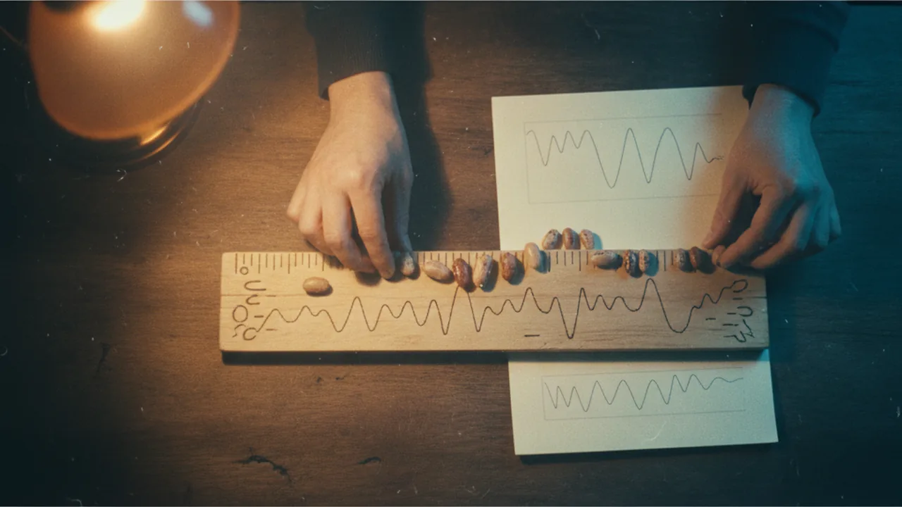
measure a continuous trait in a sample of seeds, summarize it with a histogram, mean and standard deviation, and explain the distribution with polygenic inheritance and environmental effects.
- I can use statistics and probability to analyze data about traits in a population.
- I can determine how environmental factors are related to how often a trait appears in a population using statistical analysis.
- I can use patterns in statistical data to predict how the distribution of a trait might change if the environment changes.
- I can explain whether the variation of a trait is caused by or just related to an environmental factor, using reliable evidence.
- I can identify the types and number of sources I use as evidence.
- I can evaluate whether my evidence is sufficient to support my claim and to tell the difference between cause and correlation.
- I can judge the validity and reliability of the evidence I use.
Phase 3: Make Sense
Warm-Up ~5 min
Do Now. Line up ten beans from shortest to longest. Do they fall into two or three clear groups, or a smooth range?
You measure 90 beans from one bag and graph their lengths. What shape will the histogram most likely have?
Instruction ~10 min
Not every trait comes in two types. Kernel color is purple or yellow. But seed length, human height and the sugar content of a tomato come in a smooth range of values. These are continuous traits, and most of them are polygenic: influenced by many genes, each adding a small effect, and by the environment.
Worked example 1: a model with three genes. Suppose seed length is controlled by three genes, each with an allele that adds length (capital letter) and one that does not. A plant that is AaBbCc crossed with another AaBbCc can produce offspring with 0 to 6 “adding” alleles. Each offspring gets 6 alleles, each with a 1/2 chance of being an adding allele, so the number of offspring in each class follows the pattern 1 : 6 : 15 : 20 : 15 : 6 : 1 out of 64. Few offspring are very short or very long; most are in the middle. The more genes involved, the smoother the curve. Add environmental effects, such as how much water or sun each plant got, and the bars blur into the familiar bell-shaped normal distribution.
Worked example 2: summarizing a sample (illustrative data). A class measured 30 dried pinto beans with a ruler to the nearest 0.1 mm. The shortest was 12.9 mm and the longest 17.2 mm. The mean was 15.15 mm and the median 15.15 mm, nearly equal, which is typical of a symmetric distribution. The standard deviation, which measures how spread out values are around the mean, was 0.98 mm. Grouped into 1-mm bins starting at 12.5 mm, the counts were 1, 6, 12, 8 and 3: a single peak in the middle, with tails on both sides. In a normal distribution about 68% of values fall within one standard deviation of the mean; here 21 of 30 (70%) fell between 14.17 and 16.13 mm, and 28 of 30 (93%) within two standard deviations.
| Bin (mm) | 12.5–13.5 | 13.5–14.5 | 14.5–15.5 | 15.5–16.5 | 16.5–17.5 |
|---|---|---|---|---|---|
| Count (illustrative) | 1 | 6 | 12 | 8 | 3 |
Worked example 3: genes or environment? A histogram cannot by itself tell you why seeds differ. Compare two groups grown from the same seed stock, one in full sun and one in shade (illustrative data, 8 seeds each): sunny mean 15.94 mm, shady mean 14.43 mm. Because the seeds came from the same stock, a difference of 1.5 mm, much larger than the standard deviation of either group (0.45 and 0.37 mm), points to an environmental effect. Two cautions about cause: if the sunny bed also had richer soil, light and soil are confounded, so we cannot say which one caused the difference; and eight seeds per group is a small sample. A correlation between sun and size is not yet proof that sun caused it. Some traits show the environment plainly: the same hydrangea plant makes blue flowers in acidic soil and pink flowers in alkaline soil. Geneticists say the phenotype depends on the genotype and the environment.
Predicting change. If the environment shifts, the whole distribution can shift. If next season the library’s beds were shaded all summer, the shady-group data predict the mean would move down by about 1.5 mm while the bell shape stayed similar, because the genes in the seed stock have not changed. That is a prediction to test, not a fact.
Using a simulation. The PhET Plinko Probability sim drops balls through rows of pegs; each peg is a 50-50 chance, like each allele. The pile at the bottom approaches a bell curve, the same mathematics as a polygenic trait.
Lab procedure: measuring variation in bean seeds. Question: what is the distribution of seed length in a sample of dried beans, and what does its shape suggest about the genes and environment behind it?
- Take a random scoop of 30 beans without choosing by size.
- Measure each bean’s length along its longest axis to the nearest 0.1 mm (or 0.5 mm with a ruler). Record every value.
- Calculate the mean, median, range and standard deviation (use a spreadsheet for the standard deviation).
- Group the lengths into 1-mm bins and draw a histogram. Mark the mean and one standard deviation on each side.
- Count how many beans fall within one and two standard deviations of the mean, and pool your data with two other groups to redraw the histogram with 90 beans.
| Bean | Length (mm) | Bean | Length (mm) | Bean | Length (mm) |
|---|---|---|---|---|---|
| 1 | 11 | 21 | |||
| … | … | … | |||
| 10 | 20 | 30 |
Summary: mean ___, median ___, range ___, standard deviation ___, % within 1 SD ___.
No beans? Use the illustrative data set of 30 bean lengths your teacher provides and the Plinko sim. It earns full credit.
Reading: OpenStax Biology 2e, chapter 13, Modern Understandings of Inheritance, and OpenStax Concepts of Biology, chapter 8 (CC BY 4.0); NHGRI Talking Glossary entry for polygenic trait (public domain).
Guided Exercises ~15 min
Use your measurements and the illustrative data.
Independent Practice ~10 min
Plan a test of cause.
Propose an experiment to separate genetic and environmental effects on bean length. Name the variables you would change and control, the sample size, and how you would tell a cause from a mere correlation. Then identify two sources of measurement error and their likely effect on the standard deviation.
Closure ~5 min
Next lesson, we pull together every source of variation into one explanation.
Exit ticket: why is seed length a bell curve and kernel color two classes? Use the words polygenic and environment.
How confident are you that you can summarize a continuous trait with a histogram, mean and standard deviation and explain its distribution.
Teacher notes
Materials: a bag of dried pinto or lima beans (30 per group), clear millimeter rulers or vernier calipers, graph paper or a free spreadsheet (such as CODAP), devices for the PhET sim, coins for the backup.
Timing: this workshop spans two 50-minute periods: measuring and summarizing on day 1, sim, pooling and modeling on day 2.
Listen for: “the biggest beans have the best genes”; correlation read as cause; bins of different widths. PhET link: confirm the Plinko Probability sim loads on school devices before class; the coin toss is the backup.
Support / stretch: give a spreadsheet with formulas ready and a histogram template. Stretch: build the four-gene version of the class pattern (1 : 8 : 28 : 56 : 70 : 56 : 28 : 8 : 1 out of 256) and compare its shape with the three-gene model.