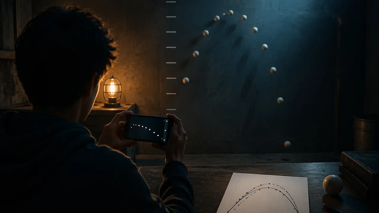
collect data on a real projectile, fit and graph a quadratic model, interpret its features, and compare it with the physics model in a written report and presentation.
Instruction
In this task you check the physics model from Lesson 3.4 against something you launch and film yourself.
1. Get a launch. All three routes earn full credit, and all three support every part of this task.
- Route A — Film your own. Film a ball tossed upward, a basketball shot or a water-fountain arc with a phone held still, with a measured scale in the frame, such as a meter stick or a wall marked in known heights. Film from far enough away that the whole path is visible and the camera is roughly level with the middle of the path. Many phones can record in slow motion, which helps. Safety first: toss soft balls outdoors, away from people and windows. Then extract the data as step 2 describes.
- Route B — The printed launch record (illustrative data built for this task). A softball tossed upward and filmed at 30 frames per second against a wall marked in meters, with a height read every three frames. No phone, no internet and no materials needed; skip to step 3.
These are real video readings in the sense that matters here: they carry the errors real readings carry, and the leading coefficient you fit will not come out at −4.9. Explaining the gap is step 5, and it is worth as much credit as a clean fit.Time t (s) 0.0 0.1 0.2 0.3 0.4 0.5 0.6 0.7 0.8 0.9 1.0 Height h (m) 1.23 1.81 2.27 2.58 2.83 3.03 3.12 3.12 2.95 2.74 2.51 - Route C — Generate a launch in the PhET simulation. Open Projectile Motion (
https://phet.colorado.edu/sims/html/projectile-motion/latest/projectile-motion_all.html), set the cannon height and angle, turn air resistance off, fire, and use the tape measure and the time-height readout to record 8 to 12 points. Then fire the same shot again with air resistance on and note how the path changes; that observation feeds step 5.
2. Extract data (Routes A and C). Step through the video or the sim frame by frame. Every few frames, record the time and the ball’s height using the scale. At 30 frames per second, each frame is 1/30 of a second. Aim for 8 to 12 data points from release to landing or catch. Free video-analysis tools, or pausing and reading heights off the screen, both work.
3. Graph and fit. Enter the data in Desmos and fit y1 ~ a x1^2 + b x1 + c. Record a, b and c. This is the same least-squares idea you used for lines in Algebra 1A, now with a quadratic. Plot the residuals and check that they show no strong pattern.
4. Interpret. Convert your model to vertex form using the graph or technology: the vertex gives the maximum height and when it happened. Interpret the y-intercept (height at t = 0, which depends on when you started the clock) and the t-intercepts (when the ball would reach the ground). State the domain on which the model applies.
5. Compare with physics. If time is in seconds and height in meters, gravity predicts a ≈ −4.9. How close is your a? Give a percent difference and explain sources of error: the camera angle, reading the scale, frame timing and air resistance, which matters more for light objects. Compare your model with the Lesson 3.4 model given as an equation: which ball went higher, and which stayed in the air longer?
6. Transformations. Describe your model as a transformation of y = x2: stretch, reflection and shifts.
The report and presentation. Write 600-900 words with your data table, a graph of the data with the model, the fitted equation in two forms, interpretations, the comparison with physics and error analysis. Present in three to four minutes, live or recorded, and defend your model when asked why your value of a differs from −4.9.
📖 Read for this lesson
The reading opens over the lesson; close it to come back to exactly where you were. The checks below draw on it.
Formative check
Work through these before moving on. They are not graded — they tell you whether the standard below has landed yet.
A fitted model with t in seconds and h in meters has a = −4.2. What is the most reasonable explanation?
In vertex form a(t − h)² + k, the maximum height of the ball is and it occurs at time .
How confident are you that you can fit, graph and interpret a quadratic model for a real projectile and compare it with physics?
Unit 3 checkpoint
Do this before you start the task. It covers the whole unit and tells you what to review first.
First differences 19, 17, 15, 13 suggest a function that is…
With 40 m of fence, the maximum rectangle area is m².
Expand (x + 3)(x − 5).
(x + 5)² = x² + 25.
The product of two polynomials is always a polynomial.
The vertex of y = −2(x + 1)² + 8 is…
Compared with y = x², y = (x − 4)² + 1 is moved…
−2(x + 1)² + 8 in factored form is −2(x − 1)(x + ).
h(t) = −4.9t² + 14.7t + 2 reaches its maximum at t = s.
In h(t) = −4.9t² + 14.7t + 2, the 14.7 is…
R(p) = p(600 − 20p) is greatest at p = .
f(x) = x² + 5 is an even function.
Submit: Launch Lab report (600-900 words with data, graph and model) and presentation
Task: Record a real projectile, extract time-height data, fit and graph a quadratic model, interpret its vertex, intercepts and domain, and compare the leading coefficient with the gravity model, explaining the difference.
Submission workflow
- Stage 1 — Plan. Your route (A, B or C) and its data; for Route A, the filming setup with scale and a safety plan; for Routes A and C, how you will extract the points; for Route B, your reading of what the printed record measures and in what units.
- Stage 2 — Peer-reviewed draft. A partner re-checks three of your data points (re-reading them from your video or sim, or recomputing three predicted heights from your model for Route B) and checks your vertex interpretation; submit a revision note.
- Stage 3 — Revised final. Data table, graph with model, standard and vertex forms, interpretations, physics comparison and error analysis, in 600-900 words.
- Stage 4 — Presentation and defense. Three to four minutes, live or recorded, defending your value of a.
How it is scored
| Criterion | What proficient looks like |
|---|---|
| Data (A1.NQ.B.3) | Time and height data extracted carefully with units and a stated scale; at least 8 points. |
| Graph and features (A1.IF.C.7) | Accurate graph of data and model, with vertex and intercepts identified. |
| Fitted model (A1.DS.A.5) | Quadratic fitted with technology, residuals checked, model written in two forms. |
| Interpretation (A1.IF.B.3, A1.BF.A.1) | Vertex, intercepts, domain and transformations interpreted correctly in context. |
| Physics comparison (A1.LQE.A.3, A1.IF.B.3, A1.IF.C.9) | Leading coefficient compared with −4.9 using a percent difference; comparison with the equation model; sources of error explained. |
| Defense (MP.4) | Presentation explains and defends the model’s fit and limits. |
Checking the Launch Record: The Fit, the Residuals, and Why a Is Not 4.9
The launch record printed in Lesson 3.5 is constructed teaching data and is illustrative; the least-squares fit, residuals and percent difference below were computed from it · SLS original (constructed teaching data, with computed fit statistics)
Why this reading. The task asks you to fit a quadratic, plot residuals, and defend a leading coefficient that will not equal −4.9. Route B students have a printed record but no way to know whether their fit is right, and a defense of a number you are not sure you computed correctly is not a defense. This reading gives the answer for Route B’s data, so you can check your own work, and one further record for the comparison the task asks for.
The Route B record, restated
A softball tossed upward, filmed at 30 frames per second against a wall marked in meters, height read every three frames. Constructed for this task and labeled illustrative.
| t (s) | 0.0 | 0.1 | 0.2 | 0.3 | 0.4 | 0.5 | 0.6 | 0.7 | 0.8 | 0.9 | 1.0 |
|---|---|---|---|---|---|---|---|---|---|---|---|
| h (m) | 1.23 | 1.81 | 2.27 | 2.58 | 2.83 | 3.03 | 3.12 | 3.12 | 2.95 | 2.74 | 2.51 |
The least-squares quadratic, and how to know yours is right
Fitting h = at² + bt + c to all eleven points gives, to three decimals:
| a | b | c |
|---|---|---|
| −4.647 | 5.877 | 1.251 |
If your technology gives you these three numbers, your data entry was correct. If it does not, check your table before you check your physics.
Vertex. t = −b ÷ 2a = −5.877 ÷ (2 × −4.647) = 0.632 s, and h there is 3.109 m. Compare that with the record itself, which shows 3.12 m at both 0.6 s and 0.7 s — two equal readings straddling the peak, exactly as symmetry predicts, with the true maximum between them and slightly lower than either would suggest once the fit smooths the reading error.
Vertex form. −4.647(t − 0.632)² + 3.109.
The residuals
Observed height minus fitted height, in meters:
| t | 0.0 | 0.1 | 0.2 | 0.3 | 0.4 | 0.5 | 0.6 | 0.7 | 0.8 | 0.9 | 1.0 |
|---|---|---|---|---|---|---|---|---|---|---|---|
| Residual (m) | −0.021 | +0.018 | +0.030 | −0.016 | −0.028 | +0.003 | +0.016 | +0.033 | −0.028 | −0.036 | +0.029 |
Every residual is under 4 centimeters, and the signs change back and forth rather than running all one way in the middle and the other way at the ends. That is what “no strong pattern” looks like, and it is the evidence that a quadratic is the right shape here. A residual plot that curved would mean the model was wrong; these only mean the readings were imprecise, which is a different and much smaller complaint. Four centimeters is about what reading a ball’s top edge off a wall scale in a video frame will cost you.
Why a = −4.647 and not −4.9
The percent difference is (−4.647 − (−4.9)) ÷ (−4.9) = 0.253 ÷ 4.9 = 5.2%, with the fitted value smaller in size than gravity predicts. Four explanations are worth weighing, and your report should rank them rather than list them:
- Perspective. If the camera is not level with the middle of the path, heights near the top of the frame are systematically misread, which bends the fitted curve.
- Scale reading. Each height is read to the nearest centimeter or two off a wall marking; the residuals above show about that much scatter.
- Frame timing. Thirty frames per second is nominal; a phone’s real frame interval can drift, and an error in t enters a squared.
- Air resistance. It always reduces the size of the fitted leading coefficient, and it matters more the lighter the object. For a softball over one second it is a small effect, so it cannot carry the whole 5.2% on its own.
What is not an explanation: gravity did not change, and how hard the ball was thrown affects b, not a.
The comparison the task asks for
Lesson 3.4’s ball was given as an equation rather than measured: h(t) = −4.9t² + 14.7t + 2, with vertex (1.5, 13.025) and landing at about t = 3.13 s. The Route B softball peaks at 3.109 m after 0.632 s. So the Lesson 3.4 ball goes more than four times as high (13.025 m against 3.109 m) and takes more than twice as long to get there (1.5 s against 0.632 s). It was thrown far harder, which is a statement about b; and both leading coefficients are set by gravity, one at exactly −4.9 and one within about 5% of it, which is a statement about the planet. Say both, in those terms.