decide with evidence whether a real data set is better modeled by a linear or an exponential function, interpret the chosen model’s parameters, and communicate its predictions and limits.
Instruction
Real data never follow a formula exactly. This task asks you to decide which kind of function describes a real pattern best, and to defend that decision.
Choose a data set. All three earn full credit, and all three support every part of this task.
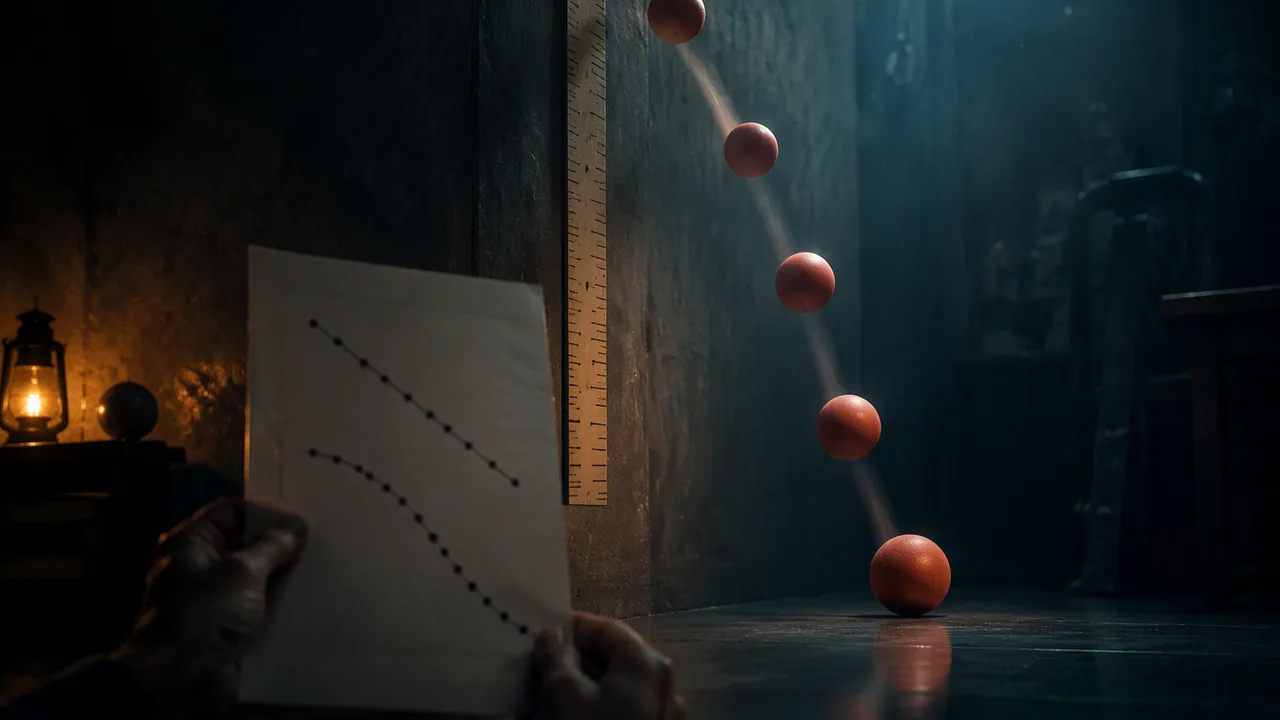
- Option A — Collect your own: bouncing ball. Tape a measuring tape to a wall. Drop a ball from a measured height onto a hard floor and record the height of each rebound, reading the top of the ball at the peak; a phone video played back frame by frame makes the peaks easy to catch. Five or six rebounds are enough. Record the ball, the drop height and the floor surface. Do this away from people and windows.
- Option B — The printed cooling record (illustrative data built for this task). A cup of hot tap water in a room held at 21.0 °C, measured every two minutes for thirty minutes. No materials and no internet needed.
Model the difference between the water and the room, not the temperature itself. Check your work: those differences are 50.0, 44.0, 38.7, 34.1, …, and each is close to 0.88 times the one before, while the consecutive differences of the temperature itself (−6.0, −5.3, −4.6, −4.1, …) shrink steadily, which is how you know the change is not linear.Minutes 0 2 4 6 8 10 12 14 16 18 20 22 24 26 28 30 Water °C 71.0 65.0 59.7 55.1 51.0 47.4 44.2 41.4 39.0 36.8 34.9 33.3 31.8 30.5 29.4 28.3 - Option C — The public record: a state’s population. Use the decennial census counts for Missouri, or for another state, published by the U.S. Census Bureau (census.gov), for a span of decades you choose. State the decades and the page you took them from. This lesson’s reading prints one fast-growing state’s twelve counts, 1910 to 2020, if you would rather work offline. These are real counts, so expect a messier fit than the other two options give.
Record the source or method, units and date for whichever option you take. Use care with hot water if you do your own version of Option B: tap water is hot enough.
Test the pattern. With equally spaced inputs, compute consecutive differences and consecutive ratios. Which is closer to constant? For the ball, the ratio of each rebound to the one before is often fairly steady, which points to exponential decay. For the census counts, look at whether the percent growth per decade stays steady over the span you chose.
Fit both models. In Desmos, type your data as a table and fit both y1 ~ m x1 + b and y1 ~ a b^(x1). Record both equations and compare the residuals: a model whose residuals show a clear pattern, such as all positive in the middle and negative at the ends, is the wrong kind. Choose the better model using three kinds of evidence: the difference and ratio patterns, the residuals and the context. Would you expect this quantity to change by a constant amount or a constant percent?
Interpret. For an exponential model, state the initial value with units and convert the factor to a percent rate per unit: a factor of 0.72 per bounce means each rebound is about 72% of the previous one, a 28% loss per bounce. If a different time unit would be more natural, rewrite the model to show it, as in Lesson 2.3.
Predict, with limits. Make one prediction slightly beyond your data and report it to a precision your measurements support. Then explain when the model will fail: a ball eventually stops bouncing, water cannot cool below room temperature, and population growth depends on births, deaths and migration that change over time. A model is a tool for a range, not a law of nature.
The report and presentation. Write 600-900 words with the data table, both fitted models, a graph and residual comparison, your choice with its evidence, the interpreted parameters and your prediction with limits. Present in three minutes, live or recorded, and answer one question about why you rejected the other model.
📖 Read for this lesson
The reading opens over the lesson; close it to come back to exactly where you were. The checks below draw on it.
Formative check
Work through these before moving on. They are not graded — they tell you whether the standard below has landed yet.
A rebound model is h(n) = 150(0.72)^n, with h in cm after n bounces. What does 0.72 mean?
If consecutive are roughly constant the data suggest a linear model; if consecutive are roughly constant they suggest an exponential model.
How confident are you that you can choose between linear and exponential models for real data and defend the choice?
Unit 2 checkpoint
Do this before you start the task. It covers the whole unit and tells you what to review first.
Which is exponential?
Linear functions change by equal differences over equal intervals.
8^(2/3) = .
2^(−3) = 1/.
Explicit rule for 3, 6, 12, 24, …?
In 500(0.92)^t, each unit of time the amount…
15% a year is about what monthly rate?
For M(t) = 200(0.5)^(t/6), M(12) = .
The exponential through (2, 180) and (4, 405) has b = .
An exponential function ab^x with a > 0 has an x-intercept.
$1,000 + $100/year versus 5%/year from $1,000: the exponential first leads in year…
A factor of 1.035 means 35% growth per unit.
Submit: Exponential or Not? model report (600-900 words with data, models and residuals) and presentation
Task: Collect or download a real data set, test it for linear and exponential patterns, fit both models, choose and defend one, interpret its parameters as a percent rate, and make a prediction with its limits.
Submission workflow
- Stage 1 — Plan. Data choice, collection method or source, units, and a prediction of which model will fit with a reason.
- Stage 2 — Peer-reviewed draft. A partner recomputes two ratios and checks your percent-rate interpretation; submit a revision note.
- Stage 3 — Revised final. Data, differences and ratios, both fitted models, residual comparison, chosen model with interpretation, prediction and limits, in 600-900 words.
- Stage 4 — Presentation. Three minutes, live or recorded, answering a question on the rejected model.
How it is scored
| Criterion | What proficient looks like |
|---|---|
| Pattern evidence (A1.LQE.A.1) | Differences and ratios computed and used correctly to argue for linear or exponential change. |
| Model construction (A1.LQE.A.3, A1.LQE.B.4, A1.DS.A.5) | Both models fitted with technology and recorded correctly. |
| Interpretation (A1.IF.B.6) | Initial value and factor interpreted in context, with the factor converted to a percent rate. |
| Graph and comparison (A1.IF.C.7, A1.LQE.A.2) | Graph shows data and model with intercept and end behavior; linear and exponential behavior compared. |
| Prediction and precision (A1.NQ.B.5) | Prediction reported to a justified precision, with the model’s limits explained. |
| Argument (MP.3) | Choice defended with three kinds of evidence; presentation answers the question on the rejected model. |
One State, 1910 to 2020: Twelve Census Counts, Their Differences and Their Ratios
U.S. Census Bureau, Historical Population Change Data (1910-2020), released Apr. 26, 2021, state FIPS 06; cross-checked against Historical Population Density Data (1910-2020); retrieved Sept. 23, 2026 · Public domain (works of the United States government), with SLS worked calculations
Why this reading. Option C of the performance task sends you to census.gov for a state’s decennial counts. One state’s counts — one fast-growing western state — are printed here, so Option C can be done with no internet, and so that everyone arguing about the data is arguing about the same numbers. They are cross-checked against a second Census Bureau table, which lists the identical twelve figures.
The counts
Resident population of one fast-growing western state (Census Bureau state FIPS code 06) at each decennial census. The differences and ratios are computed from the counts; the counts themselves are as the Bureau printed them.
| Census year | Resident population | Change from previous census | Ratio to previous census |
|---|---|---|---|
| 1910 | 2,377,549 | — | — |
| 1920 | 3,426,861 | +1,049,312 | 1.441 |
| 1930 | 5,677,251 | +2,250,390 | 1.657 |
| 1940 | 6,907,387 | +1,230,136 | 1.217 |
| 1950 | 10,586,223 | +3,678,836 | 1.533 |
| 1960 | 15,717,204 | +5,130,981 | 1.485 |
| 1970 | 19,953,134 | +4,235,930 | 1.270 |
| 1980 | 23,667,902 | +3,714,768 | 1.186 |
| 1990 | 29,760,021 | +6,092,119 | 1.257 |
| 2000 | 33,871,648 | +4,111,627 | 1.138 |
| 2010 | 37,253,956 | +3,382,308 | 1.100 |
| 2020 | 39,538,223 | +2,284,267 | 1.061 |
What the two tests say
Neither column of tests is constant, so neither a linear nor an exponential model fits the whole span. But the ratios are not random: from 1950 onward they fall almost without interruption — 1.533, 1.485, 1.270, 1.186, 1.257, 1.138, 1.100, 1.061. This state’s growth rate has been decreasing for seventy years, even while its population kept rising. That is the finding, and a report that says only “the data are exponential” has not looked at the last column.
The extrapolation that goes wrong
Fit an exponential model to 1940–1960 alone. The two decade ratios there are 1.533 and 1.485, averaging about 1.5, so a student in 1960 might reasonably write P(d) = 15,717,204(1.5)d with d in decades after 1960. Run it to 2020, six decades on: 1.56 = 11.39, so the model predicts about 179,000,000 residents. The actual 2020 count was 39,538,223. The model overshoots by a factor of more than four.
Nothing was wrong with the arithmetic. What was wrong was the assumption that a factor measured over two decades stays fixed for six. An exponential model extrapolates its own growth rate, so it is exactly as trustworthy as that rate’s stability — and this one’s was not stable. This is the concrete meaning of “explain when the model will fail” in the task.
Choosing your span, and what to report
- Choose a span of at least five censuses and say why you chose it. A short span will fit better and predict worse; say which you are optimizing for.
- Compute differences and ratios for your span, fit both a linear and an exponential model, and compare the residuals.
- Make one prediction one decade beyond your span, and report it to a precision the data support — not to the person.
- State the model’s limits using the evidence above: what happened to the growth factor, and what a falling growth factor does to any prediction made from a fixed one.
One note on the data itself. A decennial census is a count, not a sample, but it is not perfect: the Bureau publishes coverage estimates showing that some censuses missed people and others counted some twice. Treat the figures as the best available count of a hard thing to count, which is what they are, and not as exact.
Sources: U.S. Census Bureau, Historical Population Change Data (1910-2020), released April 26, 2021 (census.gov); U.S. Census Bureau, Historical Population Density Data (1910-2020) (census.gov)