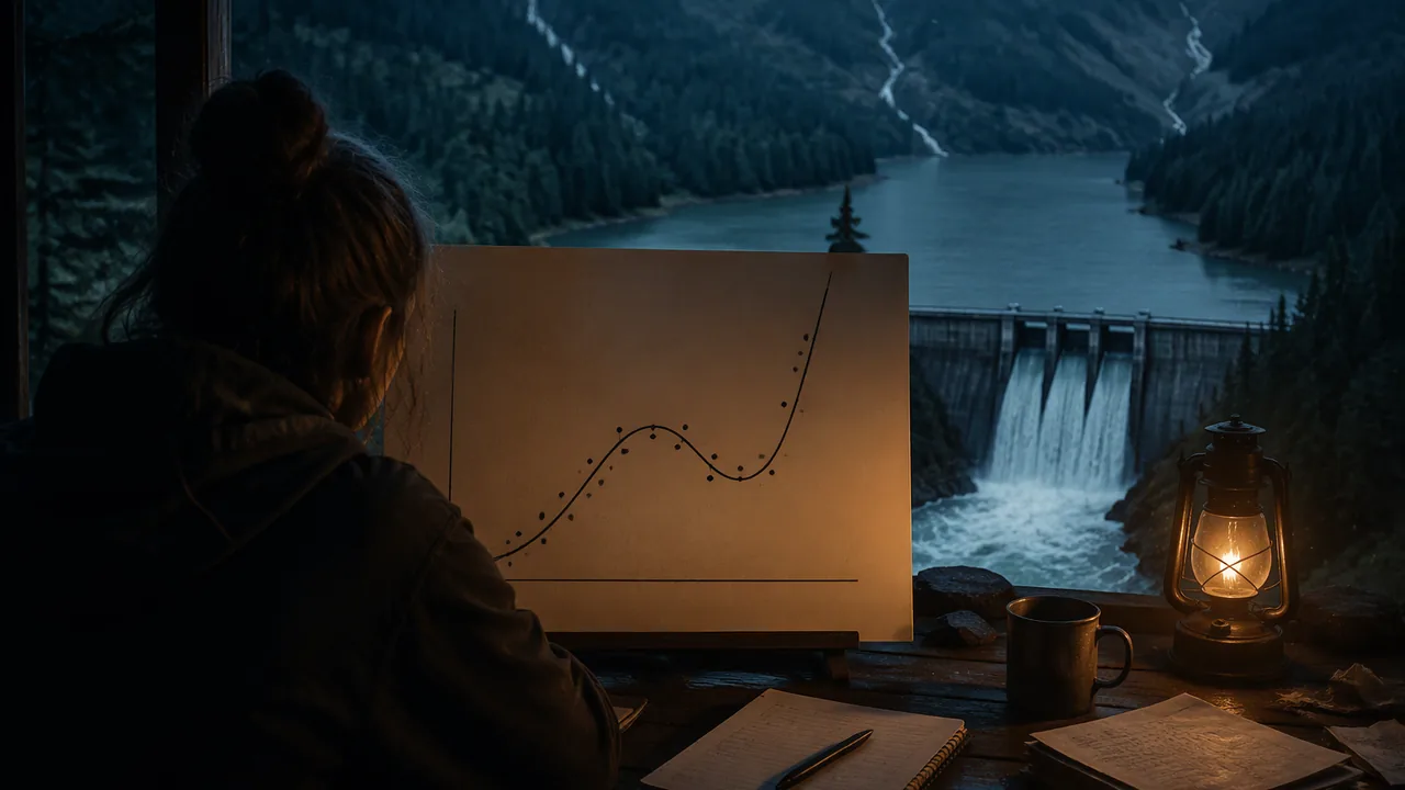
fit polynomial models to a year of reservoir storage data, interpret turning points and end behavior in context, and judge where the model can and cannot be trusted.
Instruction
Missouri’s large lakes are reservoirs behind U.S. Army Corps of Engineers dams, built mainly to hold back floods. The Corps keeps each lake near a target level, lets it rise when heavy spring rain arrives, and releases the extra water over the following weeks. It publishes daily storage for lakes such as Table Rock, Clearwater, Truman and Stockton. This lesson’s reading prints three complete water years (October through the following October) for Table Rock and Clearwater Lakes, in acre-feet and as percent of capacity; you will choose one and model it.
A worked example with illustrative numbers. The values below are invented to show the method; your data will be real. Let t = 0 be October 1 and let S be storage as a percentage of capacity.
| t | 0 | 1 | 2 | 3 | 4 | 5 | 6 | 7 | 8 | 9 | 10 | 11 | 12 |
|---|---|---|---|---|---|---|---|---|---|---|---|---|---|
| S | 40 | 38 | 42 | 50 | 60 | 70 | 78 | 82 | 78 | 68 | 58 | 48 | 42 |
Fitting by least squares with free technology (Desmos, GeoGebra or a spreadsheet) gives a quadratic with R2 ≈ 0.815, a cubic with R2 ≈ 0.903 and a quartic with R2 ≈ 0.992:
S(t) ≈ 0.0366t4 − 0.992t3 + 7.623t2 − 11.826t + 41.284.
The quartic’s relative maximum is about 79.6% at t ≈ 6.85, late April, close to the data’s peak of 82% on May 1. Its relative minimum near t ≈ 0.94 matches the November low. Those turning points have meaning: the peak is when spring inflow stops exceeding releases.
Where the model fails. The quartic has positive leading coefficient and even degree, so it rises without bound on both ends. At t = 18 it predicts about 352% of capacity, which is impossible. A reservoir cycle repeats; a polynomial cannot. That is a key finding, not a failure of your work, and your report must show it with a calculation. Higher degree always fits the data points better, but a better fit inside the data says nothing about behavior outside it.
Constraints (A2.REI.B.3). In normal operation storage stays between 0% and 100% of capacity; state these as inequalities your model must satisfy on its domain. Use the average rate of change over the months the lake rose and the months it fell to compare how fast it filled and emptied (A2.IF.A.1).
Choose one of the reservoir years in the reading, and carry its dam, data series, capacity and retrieval date into your report so anyone can reproduce your data.
📖 Read for this lesson
The reading opens over the lesson; close it to come back to exactly where you were. The checks below draw on it.
Formative check
Work through these before moving on. They are not graded — they tell you whether the standard below has landed yet.
Why does the illustrative quartic predict 352% of capacity at t = 18?
In the illustrative data, what is the average rate of change of storage from t = 1 to t = 7?
Simulation & tools
Better fit inside, worse prediction outside
Drag seven points onto the graph so they rise and then fall, like a reservoir filling and emptying. Choose Best Fit and switch between linear, quadratic, cubic and quartic, recording r2 for each. Then drag one new point to the far right edge at the same height as your first point, as if the cycle repeated, and record how each fit’s r2 and shape change. Question: which degree fit the original seven points best, and did that same fit handle the new point well? Explain using end behavior. No device: use the illustrative table in this lesson, where the quartic has R2 ≈ 0.992 yet predicts about 352% at t = 18.
Open in a new tab ↗ · PhET Interactive Simulations, University of Colorado Boulder · CC BY 4.0
Stage 1: name your lake, its dam and its capacity. Write the constraints your storage model must satisfy as inequalities, and sketch the shape you expect before fitting any model.
How confident are you that you can fit, interpret and critique a polynomial model of real data?
Unit 2 checkpoint
Do this before you start the task. It covers the whole unit and tells you what to review first.
(x + 2)(x2 − 3x + 5) = ?
Polynomials are closed under division.
End behavior of p(x) = −x4 + 3x?
At which zero does y = (x − 1)(x + 4)2 touch without crossing?
The y-intercept of y = (x − 2)2(x + 1)(x + 4) is .
The remainder when x3 − 2x + 7 is divided by x + 3 is .
If p(5) = 0, then…
A polynomial of degree 4 can have 5 different zeros.
The coefficient of x2 in (x + 2)5 is .
Which triple does the identity give for x = 4, y = 1?
Checking an equation at five values of x proves it is an identity.
A quartic fit has R2 = 0.99 on a year of reservoir data. Using it to predict two years ahead is…
Submit: Reservoir Storage Polynomial Modeling Report (4-6 pages) + 5-minute presentation
Task: Choose one of the three water years of U.S. Army Corps of Engineers storage printed in this lesson’s reading — Table Rock 2023, Table Rock 2026 or Clearwater 2017 — and copy its table into your report with the dam, data series, capacity and retrieval date. Fit quadratic, cubic and quartic models. Choose one and defend the choice. Interpret its zeros (if any in context), turning points, intervals of increase and decrease, and end behavior in terms of the reservoir, and compute the average rate of change while the lake rose and while it fell. Show with a calculation where the model gives impossible results and explain why. Connect your findings to one fact about the reservoir or the water year from a U.S. Army Corps of Engineers source.
Submission workflow
- Stage 1 — Plan. Data table with source, a hand sketch predicting the shape, the constraints on storage written as inequalities, and your three fitted models with R2.
- Stage 2 — Peer-reviewed draft. A partner reproduces one of your fits from your data and checks one interpretation; submit a revision note.
- Stage 3 — Final report. 4-6 pages with graphs, the chosen model, interpretations in context, the extrapolation failure and a limitations section.
- Stage 4 — Five-minute presentation. Present your reservoir’s year and the model’s lesson; answer two questions. A recorded presentation is an equal-credit alternative.
How it is scored
| Criterion | What proficient looks like |
|---|---|
| Key features in context (A2.IF.A.1) | Turning points, intervals and end behavior are identified correctly and interpreted in terms of storage and seasons. |
| Polynomial graphing (A2.APR.A.5) | Graphs of the fitted models are accurate and show end behavior. |
| Structure of the model (A2.APR.A.5) | Degree, leading coefficient and any real zeros are related to the graph’s shape. |
| Constraints (A2.REI.B.3) | Storage limits are stated as inequalities and used to judge the model’s valid domain. |
| Rate of change (A2.IF.A.1) | Refill and drawdown rates are computed and compared with units. |
| Tools and limits (MP.5, MP.4) | Technology is used appropriately and the extrapolation failure is demonstrated and explained. |
Three Missouri Reservoir Years, Downloaded and Fitted
USACE Corps Water Management System (CWMS) data API, office SWL: daily reservoir storage (Stor-Res, ~1Day, acre-feet) for Table Rock Dam and Clearwater Dam, value on the first of each month; capacities = storage at the top of the flood-control pool from the same system’s location levels; retrieved November 5, 2026 · Public domain (U.S. federal government data)
Why this reading. The performance task is built on a year of real reservoir storage. Three complete water years from two Missouri lakes are printed below, in acre-feet as published and as percentages of each reservoir’s capacity, with the data series names and retrieval date so anyone can reproduce or update them. Choose one and model it; the fits and turning points at the foot are the answer key, not a substitute for doing the work.
How the data are reported
Both lakes are run by the U.S. Army Corps of Engineers, Little Rock District, which publishes storage through its Corps Water Management System. Table Rock Lake is the dam on the White River near Branson; Clearwater Lake is on the Black River near Piedmont. Both are flood-control reservoirs: the Corps holds each lake near a target level, lets it rise when heavy rain arrives, and then releases the extra water over the following weeks. A water year runs October 1 to September 30, which is why every table starts in October. One acre-foot covers one acre to a depth of one foot, about 326,000 gallons. Each value is the storage on the first day of the month. Capacity here is the storage at the top of the flood-control pool (Table Rock 3,462,000 AF; Clearwater 413,700 AF), so percent of capacity says how full the lake is including the room kept empty for floods.
Table 1. Table Rock Lake, water year 2023. Capacity 3,462,000 AF
| Month | Oct 22 | Nov | Dec | Jan 23 | Feb | Mar | Apr | May | Jun | Jul | Aug | Sep | Oct 23 |
|---|---|---|---|---|---|---|---|---|---|---|---|---|---|
| t | 0 | 1 | 2 | 3 | 4 | 5 | 6 | 7 | 8 | 9 | 10 | 11 | 12 |
| Storage (AF) | 2,506,500 | 2,477,800 | 2,502,800 | 2,658,200 | 2,669,800 | 2,726,500 | 2,880,200 | 2,685,700 | 2,782,000 | 2,741,600 | 2,644,700 | 2,631,700 | 2,643,500 |
| Percent of capacity | 72.4 | 71.6 | 72.3 | 76.8 | 77.1 | 78.8 | 83.2 | 77.6 | 80.4 | 79.2 | 76.4 | 76.0 | 76.4 |
Table 2. Table Rock Lake, water year 2026. Capacity 3,462,000 AF
| Month | Oct 25 | Nov | Dec | Jan 26 | Feb | Mar | Apr | May | Jun | Jul | Aug | Sep | Oct 26 |
|---|---|---|---|---|---|---|---|---|---|---|---|---|---|
| t | 0 | 1 | 2 | 3 | 4 | 5 | 6 | 7 | 8 | 9 | 10 | 11 | 12 |
| Storage (AF) | 2,812,800 | 2,770,500 | 2,719,600 | 2,561,500 | 2,459,000 | 2,413,400 | 2,625,800 | 2,723,900 | 2,816,700 | 2,805,300 | 2,752,500 | 2,645,100 | 2,555,700 |
| Percent of capacity | 81.2 | 80.0 | 78.6 | 74.0 | 71.0 | 69.7 | 75.8 | 78.7 | 81.4 | 81.0 | 79.5 | 76.4 | 73.8 |
Table 3. Clearwater Lake, water year 2017. Capacity 413,700 AF
| Month | Oct 16 | Nov | Dec | Jan 17 | Feb | Mar | Apr | May | Jun | Jul | Aug | Sep | Oct 17 |
|---|---|---|---|---|---|---|---|---|---|---|---|---|---|
| t | 0 | 1 | 2 | 3 | 4 | 5 | 6 | 7 | 8 | 9 | 10 | 11 | 12 |
| Storage (AF) | 23,500 | 23,200 | 23,400 | 23,400 | 22,800 | 22,900 | 35,600 | 379,200 | 349,700 | 195,200 | 29,800 | 26,800 | 23,900 |
| Percent of capacity | 5.7 | 5.6 | 5.7 | 5.7 | 5.5 | 5.5 | 8.6 | 91.7 | 84.5 | 47.2 | 7.2 | 6.5 | 5.8 |
Clearwater 2017 is in this reading on purpose. For seven months the lake sits near 5.6% of capacity, its normal pool. Then the storm of late April 2017 filled it to 91.7% by May 1, and the Corps released that water over the summer. If your model is only ever tested on a year shaped like a gentle hill, you will conclude that polynomials describe reservoirs. They describe some reservoir years.
Table 4. Least-squares fits to percent of capacity
| Quadratic R2 | Cubic R2 | Quartic R2 | Quartic model | |
|---|---|---|---|---|
| Table Rock 2023 | 0.7201 | 0.7245 | 0.8405 | 0.0088t4 − 0.2153t3 + 1.4976t2 − 1.7335t + 72.2071 |
| Table Rock 2026 | 0.0690 | 0.6704 | 0.7476 | -0.0084t4 + 0.129t3 − 0.1255t2 − 3.3565t + 82.4065 |
| Clearwater 2017 | 0.2580 | 0.4828 | 0.5044 | 0.0358t4 − 1.22t3 + 11.8948t2 − 30.8141t + 15.8171 |
Table 5. What the quartics say, inside the year and outside it
Computed from the unrounded fits.
| Turning points (month, percent) | t = 15 | t = 18 | t = 24 | |
|---|---|---|---|---|
| Table Rock 2023 | min 0.67, 71.7 · max 6.56, 80.7 · min 11.22, 75.8 | 99.5% | 189.2% | 820.3% |
| Table Rock 2026 | max −2.42, 87.7 · min 4.27, 73.0 · max 9.63, 81.2 | 12.5% | −151.2% | −1,083.9% |
| Clearwater 2017 | min 1.72, −7.9 · max 7.81, 52.7 · min 16.03, −82.6 | −74.8% | −41.1% | 1,142.3% |
Three different ways to be impossible. Table Rock 2023’s quartic has a positive leading coefficient, so it climbs without bound: it passes 100% of capacity about three months after the data end and reaches 189% by t = 18, which is April of the following year. Table Rock 2026’s quartic has a negative leading coefficient, so it falls without bound: −151% by t = 18, negative water. Clearwater 2017’s quartic fails inside the year: it dips below zero between about t = 0.7 and t = 3.0 and again after about t = 11.7, because a smooth curve that has to climb to the May flood peak must swing below the flat months on either side to do it. End behavior is settled by the leading term, but a polynomial can break its constraints long before end behavior takes over.
Notice something else in Table 4. For Table Rock 2023 the quartic buys a real improvement over the cubic, 0.8405 against 0.7245, because the year has two bends. For Table Rock 2026 the jump comes earlier, from 0.069 to 0.670 between the quadratic and the cubic: the year falls through the winter, refills in spring and falls again, a shape no parabola can follow. For Clearwater 2017 even the quartic explains only half the variation (0.5044): a flood pulse is a spike, and polynomials are smooth. A jump in R2 means the extra degree captured something; a flat or low R2 means the family of curves is wrong for the data. Reporting R2 for all three degrees, as the task asks, is what makes that visible.
Table 6. Average rates of change, in percentage points per month
| Rise | Fall | |
|---|---|---|
| Table Rock 2023 | t = 1 to 6: (83.2 − 71.6) ÷ 5 = +2.32 | t = 6 to 11: (76.0 − 83.2) ÷ 5 = −1.44 |
| Table Rock 2026 | t = 5 to 8: (81.4 − 69.7) ÷ 3 = +3.90 | t = 8 to 11: (76.4 − 81.4) ÷ 3 = −1.67 |
| Clearwater 2017 | t = 6 to 7: (91.7 − 8.6) ÷ 1 = +83.1 | t = 7 to 11: (6.5 − 91.7) ÷ 4 = −21.30 |
In every year the lake rises faster than it falls, and at Clearwater the contrast is extreme: a month of rain against four months of scheduled release. Releases are planned and rain is not, and the Corps empties a flood pool deliberately so the lake is ready for the next storm. That contrast is the kind of finding the report’s interpretation section is for, and it comes from two subtractions.
The lesson’s illustrative table, checked
Lesson 2.5 works a constructed example: t = 0 to 12 with S = 40, 38, 42, 50, 60, 70, 78, 82, 78, 68, 58, 48, 42. Fitting it here gives quadratic R2 = 0.8146, cubic 0.9034 and quartic 0.9919, and the quartic is 0.0366t4 − 0.9920t3 + 7.6228t2 − 11.8264t + 41.2844 — matching the lesson to every printed digit. Its relative maximum is 79.62% at t = 6.847 and its relative minimum 36.11% at t = 0.940, and at t = 18 it returns 352.2%, the figure the lesson’s check asks you to explain. If you substitute the four-figure coefficients exactly as the lesson prints them you get 355.0% instead: rounding the leading coefficient 0.036576 up to 0.0366, an error of 0.000024, is multiplied by t4 = 104,976 into about 2.5 percentage points. Its average rate of change from t = 1 to t = 7 is (82 − 38) ÷ 6 = 7.33 percentage points per month. Confirm your own fitting tool on this known answer before you use it on a lake.
Constraints, and the source line your report needs
Storage cannot be negative, and in normal operation it does not exceed the top of the flood pool, so a model S(t) of percent of capacity is subject to 0 ≤ S(t) ≤ 100. (A lake can rise above its flood pool in an extreme flood: Table Rock reached about 103% of this capacity on May 1, 2017. Your model is not meant to predict that.) The interval of t on which your model satisfies both inequalities is its valid domain; for Clearwater 2017 that is not even the whole data year. Say so with the calculation.
Cite the data the way this reading does: lake and dam, data series, water year, capacity with its own source, and the retrieval date. The Corps revises provisional values after review, so a download in October and one in March may not agree, and only a dated citation makes that detectable. If you want another Missouri lake or year, the same system publishes them.
Sources: USACE CWMS Data API, Table_Rock_Dam-Headwater.Stor-Res.Inst.~1Day.0.MN-Stor (office SWL) (cwms-data.usace.army.mil); USACE CWMS Data API, Clearwater_Dam-Headwater.Stor-Res.Inst.~1Day.0.MN-Stor (office SWL) (cwms-data.usace.army.mil); USACE Little Rock District, water management (swl-wc.usace.army.mil)